Original Article

Affiliation:
Pharmacelera, 08028 Barcelona, Spain
Email: enric.herrero@pharmacelera.com
ORCID: https://orcid.org/0000-0001-7837-3593
Explor Drug Sci. 2023;1:388–404 DOI: https://doi.org/10.37349/eds.2023.00026
Received: February 14, 2023 Accepted: June 16, 2023 Published: October 30, 2023
Academic Editor: Walter Filgueira de Azevedo Jr., Pontifical Catholic University of Rio Grande do Sul, Brazil
The article belongs to the special issue Machine Learning for Drug Science
Aim: Solubility prediction is an essential factor in rational drug design and many models have been developed with machine learning (ML) methods to enhance the predictive ability. However, most of the ML models are hard to interpret which limits the insights they can give in the lead optimization process. Here, an approach to construct and interpret solubility models with a combination of physicochemical properties and ML algorithms is presented.
Methods: The models were trained, optimized, and tested in a dataset containing 12,983 compounds from two public datasets and further evaluated in two external test sets. More importantly, the SHapley Additive exPlanations (SHAP) and heat map coloring approaches were used to explain the predictive models and assess their suitability to guide compound optimization.
Results: Among the different ML methods, random forest (RF) models obtain the best performance in the different test sets. From the interpretability perspective, fragment-based coloring offers a more robust interpretation than atom-based coloring and that normalizing the values further improves it.
Conclusions: Overall, for certain applications simple ML algorithms such as RF work well and can outperform more complex methods and that combining them with fragment-coloring can offer guidance for chemists to modify the structure with a desired property. This interpretation strategy is publicly available at https://github.com/Pharmacelera/predictive-model-coloring and could be further applied in other property predictions to improve the interpretability of ML models.
Aqueous solubility is a key molecular property for the discovery and optimization of new drugs. In the early stage of drug discovery, low molecular solubility is a relevant attrition factor in screening assays. Moreover, solubility has an important impact on Absorption, Distribution, Metabolism, Excretion and Toxicity (ADMET) properties of drugs, like oral absorption and bioavailability [1]. With the advent of novel machine learning (ML) algorithms and libraries, the performance of such predictors has increased significantly but remains an open field of research [2].
However, there are several open questions in the generation of ML models that go beyond the predictive performance of the models themselves. One of them is model interpretability, which could provide helpful information to researchers in the lead optimization process. Many times, ML models operate as a black box, which, combined with the employment of many descriptors (> 100), makes them difficult to interpret [2–4]. While many efforts have been made to improve the accuracy of ML models, model interpretation is still under investigation. In the field of model interpretation, there are many model-dependent or -independent strategies, such as feature-based, atom-based, fragment-based, compound-based, or graph-based approaches [5]. These approaches give aid to the researchers in understanding how a change in the descriptors or the chemical structure could affect the prediction. Since solubility changes can be understood in most cases by the addition/deletion of polar or non-polar atoms, solubility models are a good benchmark set to validate interpretation methods.
Another important aspect when building ML models is the selection of the most appropriate descriptors and algorithms, since not always the most complex and novel methods are the most adequate for all application scenarios. Any increase in complexity should be justified by a significant increase in performance to compensate for the penalty in terms of usability and interpretability it will introduce.
In this work, we will focus on the assessment of which are the best descriptors and ML algorithms to generate an accurate aqueous solubility predictor and what are the best methods for interpreting it. The performance of different ML models will be compared to existing models on different test sets. And then three interpretation approaches (feature-based, atom-based, and fragment-based) will be employed to interpret the solubility model.
To compile a diverse and large dataset to build our model, two datasets with experimental aqueous solubility values (LogS) were used. The first one AqSolDB [6], consisting of 9,982 compounds, was generated by merging nine different aqueous solubility datasets. The second dataset was collected by Cui et al. [7], which includes 9,943 compounds from ChemIDplus database and PubMed search. These two datasets were then merged as the source of the training set, validation set, and test set used in this study. In addition, two external test sets were used to further evaluate the model performance [7–10], including the Drug-Like Solubility-100 (DLS-100) dataset from Mitchell et al. [10] (external test set A) and the test set collected by Cui et al. [7] (external test set B), and are composed of 100 and 62 compounds respectively.
The merged dataset was prepared using the following methodology. First, molecules containing common elements (H, C, N, O, F, P, S, Cl, Br, and I) were kept while duplicates and large compounds (molecular weight ≥ 1,000) were removed. Then, molecules with a standard deviation of LogS greater or equal to 0.5 in AqSolDB were removed. Finally, compounds with high similarity with samples in the two external test sets were also filtered for the sake of validating the model in a more objective way. Herein, highly similar compounds were defined as those having a Tanimoto similarity based on extended connectivity fingerprints (ECFP) 4 larger than 0.90. A total of 12,983 molecules were retained and then randomly split into the training set, validation set, and test set with a proportion of 60%, 20%, and 20%, respectively. Overall, a total of five datasets were employed in this study, namely the training set with 7,789 compounds, the validation set with 2,579 compounds, test set with 2,579 compounds, external test set A with 100 compounds, and external test set B with 62 compounds.
After curating the dataset, a set of physicochemical descriptors, computed with the PyDPI software [11], was used to featurize each compound. PyDPI can represent molecules by means of different types of molecular descriptors, including constitutional descriptors, topological descriptors, connectivity indices, Burden descriptors, Basak’s information indices, electro-topological state indices, autocorrelation descriptors, charge descriptors, molecular properties, kappa shape indices, and molecular operating environment-type descriptors.
Originally, a total of 614 descriptors were computed for each compound. Descriptors that had zero variance among the training set were firstly removed in this study. For further selection, a Pearson correlation pairwise analysis was performed for the descriptors and only kept one descriptor randomly if two descriptors were highly correlated (Pearson correlation coefficient ≥ 0.90). Overall, a total of 256 descriptors were kept for the next model construction and then they were scaled to range from 0 to 1 (Table S1). To visualize whether these descriptors could capture and magnify distinct aspects of chemical structures, principal component analysis (PCA) [12], which could convert high-dimensional datasets into low-dimensional space, was performed among the training set, validation set, and test set. The feature space was visually determined by plotting the first three principal components (PC).
In this study, three ML techniques were employed to build and select a good predictive model, including the random forest (RF), deep neural network (DNN), and massage passing neural network (MPNN). In addition, four other solubility models were used as references for performance evaluation.
RF [13–15] is a supervised learning algorithm that assembles many decision trees as an ensemble. The general idea of RF is to train multiple decision trees on different subsets, sampling from the original training set and then merging the prediction results of each sub-model by taking average or voting. This popular ensemble approach takes advantage of combining different learning models on random sampling and random selection of feature sets to get a more accurate and robust performance, as well as overcomes the common overfitting problem. In our study, the hyperparameters of RF were optimized based on the root mean squared error (RMSE) in the validation set. If RMSE values were the same, then the coefficient of determination (R2) metric was used. Finally, the number of trees in the forest (“n_estimators”) was 600, the number of features to consider when looking for the best split (“max_features”) was 0.2 and the out-of-bag strategy was applied (“oob_score = true”). This model was built with the scikit-learn Python library (version1.0.2) [16].
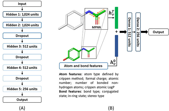
DNN [17, 18] is a feed-forward neural network that consists of one input layer, multiple hidden layers, and one output layer. Normally, the descriptors are taken into the input layer, then non-linear transformations are proceeded among the hidden layers, and finally, a prediction is produced with the output layer. Weights and biases in each layer are trained using the back-propagation technique. The architecture of the DNN model used in our study is shown in Figure 1. A total of five hidden layers were enabled in the DNN model, each of which consisted of 1,024, 1,024, 512, 512, and 256 nodes respectively. The rectified linear unit (ReLU) function was chosen as the activation function. An Adam weight optimization solver was used, and the learning rate was initialized to 0.001 and decayed with a factor of 0.8 every 5 epochs [19]. The batch gradient descent strategy was employed to train the DNN model with a maximum epoch of 300. Model optimization was performed with an early stopping strategy based on the best results in the validation set to avoid overfitting. The patience, the number of epochs to wait before an early stop if no progress on the validation set, was set to 15. Three dropout layers were used to further avoid overfitting of the DNN model. The model was built with the PyTorch framework (version 1.10.2) [20, 21].
The concept of an MPNN model [22, 23] is taking a molecule as a graph where an atom is a node, and a bond is an edge. An MPNN model usually contains three phases, an initial phase, a message-passing phase, and a readout phase. The nodes (atoms) and edges (bonds) are firstly initialized with atom features xv or bond features evw which are listed in Figure 1 and Table S2. In the message passing phase, it consists of T steps, which are set to 3 in this work. On each step t for each node v, its hidden state
The MPNN model was trained by means of the batch gradient descent method with a batch size of 128 and optimized with an Adam optimizer. The learning rate was initialized to 0.001 and decayed with a factor of 0.9 every 3 epochs. Also, the model was optimized with the early stopping strategy and whose patience parameter was set to 7. In this study, the MPNN model was implemented based on the framework of variant MPNN-S [24] and PyTorch [21].
To compare our model performance, four models were used as reference models, including two ML models built by ourselves and two other publicly available models.
The first reference model was constructed with graph convolutional (GraphConv) method [25]. Similar to the MPNN model, the GraphConv model also treats the chemical structure as a graph and represents the graph with atom-based and bond-based properties. And then convolutional and pooling layers are used to update the information of each node by aggregating the information of its connected nodes. In this study, we built a GraphConv model by applying the default implementation from the DeepChem library (version 2.4.0) [26], which contains one GraphConv layer and one dense layer, and this model was used as a reference model for later comparison. The number of training epochs was optimized based on the performance in the validation set, which was finally set to 1,500.
In addition, two public models, namely ALOGPS 2.1 [27], and ESOL equation [28], were also included for the performance comparison in this study. For the ALOGPS 2.1 it employed molecular weights and electro-topological state indices as descriptors and neural network techniques for model construction. For the ESOL equation, it is a simple linear model. This linear regression model considered four descriptors, including LogP, molecular weight, number of rotatable bonds, and proportion of heavy atoms in aromatic systems.
Furthermore, the four descriptors from ESOL equation were combined with the RF algorithm to build another reference model by ourselves [RF with ESOL descriptors (RF_ESOL)]. It was also trained in our training set and hyperparameters were optimized in the validation set. The hyperparameters “n_estimators” and “min_samples_split” of this RF_ESOL model were set to 800 and 4, respectively. Also, the scikit-learn Python library (version 0.23.0) was employed to build this regression model.
The predictive performance of our solubility models was assessed by four metrics, including R2, RMSE, %LogS ± 0.7, and %LogS ± 1.0. See Supplementary materials for the definition of R2 and RMSE. Another two metrics %LogS ± 0.7 and %LogS ± 1.0 proposed by Boobier et al. [2] have also been used and are defined below:
The %LogS ± 0.7 is defined as the percentage of compounds where the predicted LogS is in the range of experimental LogS ± 0.7. The %LogS ± 1.0 is defined as the percentage of compounds where the predicted LogS is in the range of experimental LogS ± 1.0.
The rationale of these two metrics was that an experimental error of ± 0.5–0.7 exists for aqueous LogS value in literature [29], resulting from variations in temperature, pH, and solvent purity. It would influence the reliability of R2 and RMSE in evaluating model performance as they are dependent on the range of LogS in the model. Considering the effect of experimental error, %LogS ± 0.7 could help the users understand the maximum accuracy of the model and %LogS ± 1.0 sets a limitation of the usefulness of the model for the development process.
As the test sets only contained a limited number of samples and the unavoidable experimental errors of LogS, the evaluation results may be biased. Thus, the bootstrapping method [30–32] was chosen for the analysis of the confidence interval as it is a convenient and recommended strategy to estimate the properties of estimators for any distribution with limited samples. In brief, the bootstrap sampling in our study was conducted as follows. Random sampling of 10,000 redundant copies with replacements was conducted on the test set. Each copy had the same size as the original test set. For example, the total sample size of the test set, and external test sets A and B were 2,597, 100, and 62, respectively. Then, the developed model was re-evaluated on each redundant copy of the test set with three performance metrics. As a result, an ensemble of 10,000 bootstrap samples was obtained for each performance metric, and a certain confidence interval (e.g., 95%) was derived accordingly. In this study, the percentile bootstrap method was used to compute the 95% confidence interval.
In terms of model interpretation, different methods have been evaluated such as the Shapley Additive exPlanations (SHAP) and heat map coloring. Herein, the SHAP method [33] is a feature-based interpretation method, which originated from a game theory approach [34]. It is a local interpretable approach that can explain the feature importance on an individual instance or a group of instances for any ML model. The computed SHAP value for a specific feature represents both the magnitude and direction of its contribution to the prediction. Feature with a positive sign has a positive contribution while a negative sign indicates a negative contribution to the model prediction. The work from Rodríguez-Pérez and Bajorath [35] in 2020 has shown a promising application of SHAP analysis in ML model interpretation. There are some variants for implementing SHAP and TreeSHAP [36] is used to interpretate our RF model in this study as it is a fast and tree-based model-specific method for producing feature attributions.
For the heat map coloring strategy, it is usually applied to color on the atomic or fragmental contribution to a molecular property on a two-dimensional (2D) structure, and it provides a direct interpretative visualization to the chemist. To compute the atom-level or fragment-level importance in a given prediction, those descriptors associated with an atom or fragment are removed and the change produced in a new prediction is associated to the removed atom or fragment. Thus, this method is also known as atom removal explanation. Similarity maps [37], the universal approach [38], and the atom-coloring scheme [39] are different implementations of this strategy. In this study, we followed the atom-coloring scheme framework to compute the atom or fragment contribution on a chemical structure. The protocol for atom-coloring and fragment-coloring used in this study is shown in Figure 2. Specifically, we mask each heavy atom or fragment atoms as dummy atom(s) [40] and transform bond between dummy atoms into a zero bond and the bond between non-dummy and dummy atoms into a single bond. This is different from other atom removal methods like the atom-coloring method where the removed atoms are replaced by a sodium atom. Bonds are also treated differently than in the universal approach where they propose to remove bonds between the interpretated fragment and the remaining structures. Herein, the idea of this masking strategy is that we want to account for the nonadditive effects by making the masked molecule to inherit inherent structural information (such as the links between atoms) from the reference (unmasked) molecule as much as possible. The dummy atom has “blank properties” (zero molecular weight and formal charge) which would help us minimize the inherent impact of the atom replacer on the new replacing molecule. Then we recalculate the descriptors, predict the solubility of the masked molecules and calculate the difference of predicted LogS between the masked and unmasked molecule, assigning the difference as the contribution of this atom or fragment to the molecule. The interpretation image is drawn with the open-source software RDKit [41]. Herein, we provide a script for automatically fragmenting a molecule into functional groups, rings, and other fragments and the chemist could also manually fragment it to meet their personalized study.
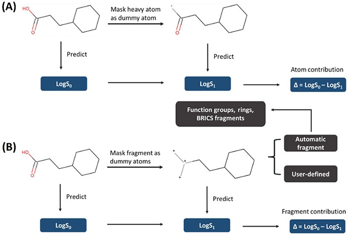
General protocol of heat map coloring. (A) Atom-coloring scheme; (B) fragment-coloring scheme
For a clearer visualization of the interpretation results, single molecule normalization was performed for all contribution values of atoms or fragments. Herein, single molecule normalization enables us to see small differences between atoms/fragments of a compound. The normalized contribution of an atom or fragment i (
If all the atomic or fragmental contributions ≥ 0, then normalize to [0, 1].
If all the contributions ≤ 0, then normalize to [–1, 0].
Otherwise, the normalization range is set to [–1, 1] (most cases).
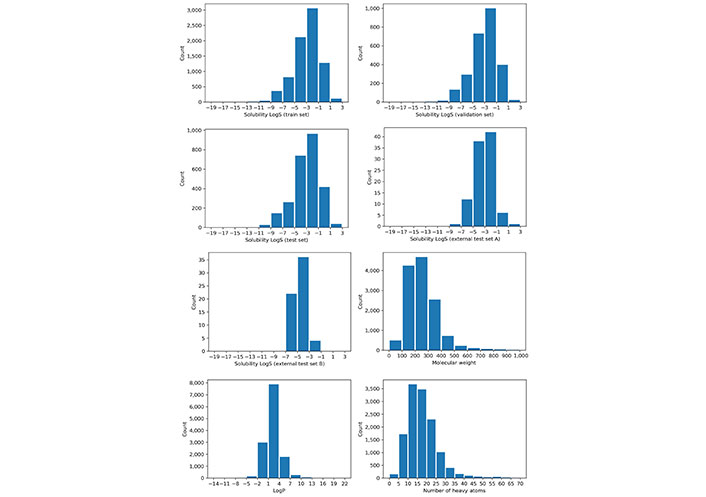
Before building the models, a property analysis was performed on the different datasets to ensure they were balanced and with a reasonable degree of variability in the solubility values. The experimental solubility (Sexp) distributions of these datasets are shown in Figure 3. A similar and diverse distribution was found among the training set, validation set, test set, and external test set A. However, external test set B has a more biased property distribution towards less soluble molecules.
A set of physicochemical descriptors were used to represent the molecule and a PCA analysis for these descriptors was also performed. The PCA analysis results are shown in Figure 4, where points have been colored based on their experimental LogS. In this study, a compound is classified as an insoluble molecule if its LogS is less than –2.0, otherwise it is considered soluble. From Figure 4, we can see that the chemical space described with the physicochemical descriptors is diverse while the partitioning of soluble and insoluble compounds is also visible. Most of the soluble molecules (blue points) are located on the inner side while most of the insoluble ones (red points) are on the right and outer side, demonstrating the ability of these descriptors to identify soluble and insoluble molecules. The PCA analysis of three datasets also shows that they share a similar distribution.
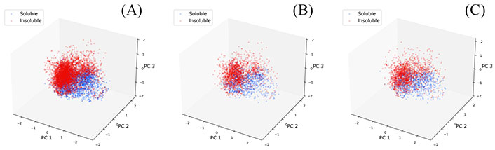
PCA analysis of descriptor space for three datasets. (A) Training set; (B) validation set; (C) test set
Three ML models were developed based on our training set with 7,789 compounds and then were evaluated on three test sets using four performance metrics. All performance results are depicted in Figure 5 and Tables S3–5. Across the three datasets, the three RF [RF with default descriptors (RF_Property)], DNN (DNN_Property), and MPNN models obtained a comparable and better performance than that from the four reference models. The RF_Property model showed a consistently excellent performance among the three test sets with different metrics. The RMSE of the four reference models in the test set were 1.06, 1.16, 1.22, and 1.04 respectively while our three developed models (RF_Property, DNN_Property, and MPNN model) in the test set were all 0.90, stating that our developed models have a better predictive ability.
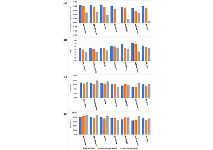
Model performance. (A) Coefficient of determination results; (B) RMSE results; (C) %LogS ± 0.7; (D) %LogS ± 1.0
The three developed ML models showed less difference in the test set than those in two external test sets. As the source of training set, validation set, and test set were randomly split from a curated dataset, they had a similar distribution and shared a system error. Thus, the external test sets were very important to assess solubility predictive models objectively. In the external test set A/B, the R2 of RF_Property, DNN_Property, and MPNN were 0.795/0.490, 0.780/0.507, and 0.744/0.361, and %LogS ± 1.0 of them were 0.850/0.887, 0.770/0.887, and 0.740/0.850, respectively. This shows that the RF_Property model is better than the DNN_Property and MPNN models. It is not surprising as tree-based models perform better on tabular-style datasets than standard deep models [36] and a systematic study from Jiang et al. [42] also demonstrated that descriptor-based models could achieve better or comparable performance in the predictions of many molecular properties. Among the external test set B, which contains 62 compounds under pH 7, the simple linear model ESOL equation got a comparable performance (RMSE was 0.64) with that from RF_Property (RMSE was 0.63) while some other ML models obtained worse results, e.g., the RMSE of MPNN and GraphConv were 0.71 and 0.90. For the other two test sets, RF_ESOL performed better than the linear model, but worse than the physicochemical descriptors with RF or DNN algorithms. These results show that descriptors and non-linear ML techniques are important for the quality of the final model.
For those compounds with absolute error larger than 1.0 (error bars in Figure 6), some recurrent substructures were found (Figure 7) such as nitrogen-containing heterocycles and aromatic systems. In the external test set B, the absolute errors of two most soluble molecules were larger than other compounds. From Figure 3, we could see that highly soluble compounds (LogS > 0.00) were less distributed in the training set, which may result in these two outliers. For the outlier with name of KEMDOW, its Crippen LogP was –1.735 which may lead to the experimental error.
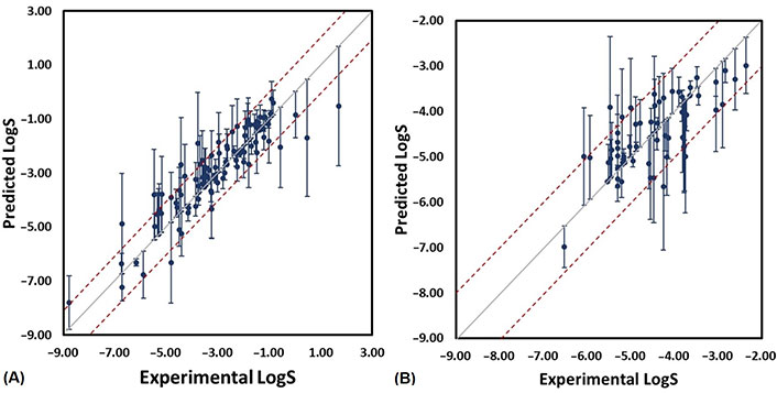
Scatter plot of experimental and predicted LogS from RF_Property model (the error bars are computed from the difference between predicted and experimental LogS). (A) External test set A; (B) external test set B
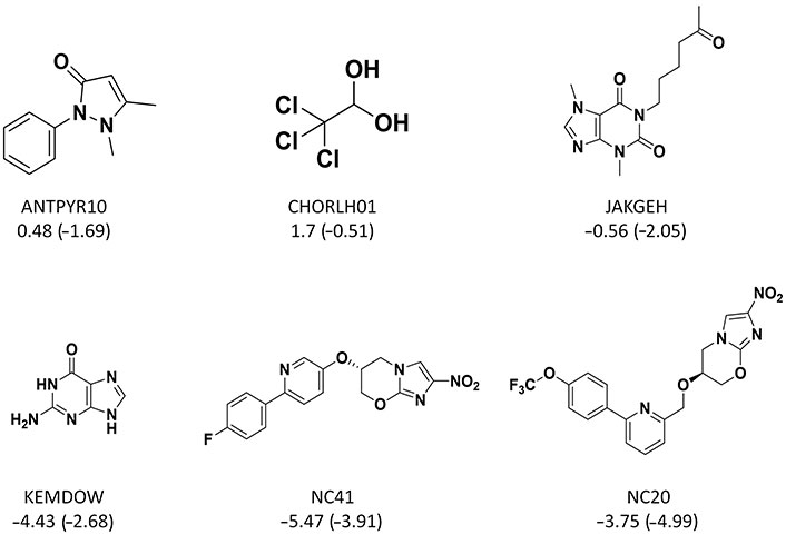
Some chemical structures of outliers. The caption under each structure is the molecule name, experimental LogS (predicted LogS from RF_Property model)
After evaluating the performance of different algorithms, the second part of this study evaluates the suitability of different interpretation methods for the best-performing algorithm, the RF_Property model.
Firstly, the TreeSHAP method was used to compute the feature importance based on 1,000 random compounds from the training set. The feature importance from TreeSHAP calculation is shown in Figure 8 and indicates that Crippen LogP (LogP) and its square (LogP2) are the most relevant descriptors in the solubility prediction and have a strong correlated relationship. The higher the LogP or LogP2 descriptor values, the lower the solubility value, which is in accordance with our intuition. Also, hydrophilic index (Hy) and some burden descriptors (bcute10, bcutm3, and bcutm4), play a role in the predictive model and their interpretation results indicate that the reduction of their values could be beneficial to improve the solubility. Interestingly, the top six most important features calibrated from Gini importance in the RF model are the same as those in the TreeSHAP method. Such descriptors could provide a simple rule of thumb for a chemist to assess the solubility of a given compound.
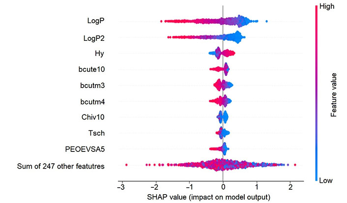
SHAP interpretation result of RF_Property model. The y-axis shows the most important features and in the x-axis we can see the computed SHAP values on 1,000 training samples. Positive value means a positive contribution while a negative one indicates a negative contribution to the model prediction
Although the feature importance method gives interesting insights on the relevance of specific molecular properties for solubility prediction it does not help chemists take direct actions to improve the solubility of a given compound as there is no information on which regions of the molecule are improving or reducing more the solubility of a given compound. Therefore, we also evaluated the suitability of the atom-coloring scheme and fragment-coloring scheme for model interpretation. As shown in Figure 9, for the compounds NC61 and NC17 of the external test set B, both strategies were capable of explaining the atomic or fragmental contribution to the molecular solubility. The carbonyl group was beneficial for the solubility while the ethylene carbons and aromatic rings made negative contributions to it. In the case of compounds C-499 and C1257 of the training set, the interpretation result of fragment-coloring scheme was more robust and reasonable than that of atom-coloring scheme. Both schemes could show the modification from carbon to hydroxy group was helpful for improving molecular solubility. The aromatic rings and carbon atoms would decrease the solubility while the hydroxy group and ester functional group were indicated to make positive contributions in both compounds from the fragment-coloring results. However, in the atom-coloring results, the contribution of aromatic rings and carbons is not consistent as the overall color is heavily influenced by the overall prediction value (highly soluble compounds will tend to paint all atoms as having a positive influence and vice versa). This phenomenon was similar to the conclusion from Sheridan’s work [39] that atom-level coloration was not robust enough and indicates that for this model, fragment-based coloring is more suitable. Therefore, in the following part, we will focus on discussing the fragment-coloring interpretation. It is worth noting that the heat map coloring and normalization method only consider the difference within the molecule. We should focus on the relative values of the intramolecular contribution, and it was not fair to compare intermolecular atomic or fragmental contribution which was dependent on the molecule.
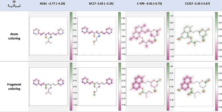
Example of atom- and fragment-coloring scheme. The caption of each structure is the molecule name, experimental LogS (predicted LogS from RF_Property model). Spred: predicted solubility
The second example of fragment-coloring scheme includes the six poly-ADP-ribose-polymerase (PARP) inhibitors designed by Johannes et al. [43]. In their work, they applied structure- and property-based strategies for drug design and observed a series of compounds that showed excellent efficacy to the target. And they also measured aqueous solubility under pH 7.4 condition for some of the active compounds, which provides good examples for interpretation in our study. The interpretation results for six compounds (all of them are excluded in the datasets for model construction of this study) from the fragment-based coloring strategy are shown in Figure 10. Their most relevant SHAP descriptors and atom-coloring results are also shown in Table S6 and Figure S1 respectively. As we could see, our RF_Property model has a good predictive ability for most of compounds and the interpretation results are consistently stable. These six compounds shared the same scaffold and the modified substructures ranged from an aromatic ring to an ethyl group. As we can see from Figure 10, the shared piperazine and imidazole fragments were proposed to make positive contribution to the Spred whereas the fragments themselves were soluble in water. The shared benzene was proposed to make most of the negative contribution to the Spred. For the highly insoluble (predicted LogS ≤ 4) compounds P10–P12, the modified part, which was benzene, pyridine, and cyclohexene ring, was predicted to hinder or hardly affect the molecular solubility. And the other modification in slightly insoluble (–4 < predicted LogS ≤ –2) compounds P13–P15 made positive or almost zero contribution to solubility improvement. It is also interesting to see that replacing a carbon with a nitrogen or oxygen within the ring system was helpful to improve the solubility. For example, the contribution of modified benzene ring in P10 was similar to the fixed benzene, while the pyridine ring was less negative than the fixed benzene within the P11 compound. Such a similar phenomenon was also observed in compounds P12, P13, and P14. In general, the interpretation results in Figure 10 were in line with instinctive chemical knowledge, showing a good interpretation power of our model and fragment-based coloring method. Non-normalized results can be found in Figure S2 and the same color distribution but with different intensities for different molecules depending on the Spred value is shown.
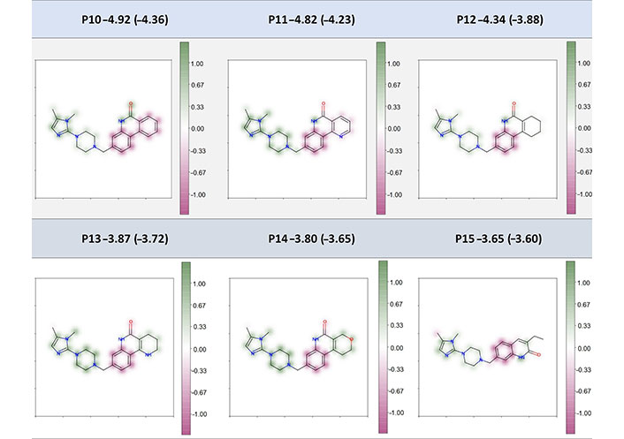
Fragment-coloration results of six PARP inhibitors. The caption of each structure is the molecule name, experimental LogS (predicted LogS from RF_Property model)
Previous examples highlight standard modifications that could be applied by a chemist to improve the solubility with the addition of more polar atoms. In our study, four “abnormal” compounds not present in the training or validation sets were also used to validate the interpretability of our model. Three of these molecules are immunomodulatory drugs, namely thalidomide, lenalidomide, and pomalidomide, and the fourth (EM-12) is a related derivative extracted from [44]. For these four compounds, replacing a methylene with a carbonyl group was reported to decrease the molecular solubility, which is against our chemical intuition to some extent. The theoretical study stated that the carbonyl group could have an extended π-conjugation with carbonyl groups of the right part through the nitrogen and such an extended π-electron led to a lower solubility. Our interpretation results (Figure 11) showed that the carbonyl groups in thalidomide and pomalidomide were proposed to make negative contribution to the Spred while the carbonyl groups in EM-12 and lenalidomide contributed positively, in line with the prospective that the modification from one carbonyl to methylene could make a positive contribution to the Spred by hindering the internal π-conjugation. On the other hand, if we compare thalidomide and pomalidomide, the addition of an amine group was proposed to make a negative contribution to the Spred. The intramolecular hydrogen bond formed by the amine and the nearest carbonyl oxygen would be unfavorable which was supported by the experimental solubility value. This added amine group was shown to make zero contribution in the lenalidomide, and its experimental and Spred were almost the same as that of EM-12.
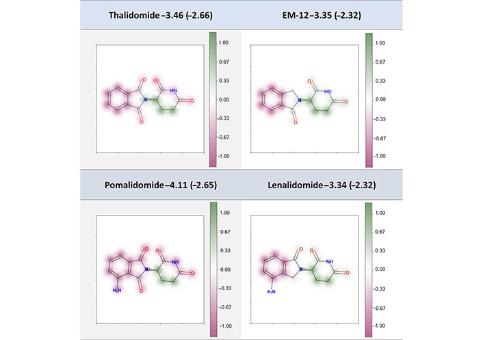
Fragment-coloration results of four compounds. The caption of each structure is the molecule name, experimental LogS (predicted LogS from RF_Property model)
In this study, several ML models for predicting aqueous solubility of small molecules have been proposed and evaluated. From all the evaluated algorithms and descriptors, the RF_Property model, combining physicochemical descriptors and RF technique, has obtained the best performance among three different test sets assessed by different metrics.
From the interpretation perspective, we have shown that feature importance extraction provides valuable information on the most relevant descriptors and showed that LogP and Hy descriptors play an important role in solubility prediction.
Feature importance, however, does not directly help the ligand optimization process which can benefit more from the extraction of heat map coloring. In this area, we have shown that fragment-based coloring offers a more robust interpretation than atom-based coloring and that normalizing the values further improves it. Such visualization can offer guidance for chemists to modify the structure with a desired property. This strategy has been evaluated in the domain of solubility prediction but could also be applied and validated in other research fields, such as activity prediction and ADMET property prediction, to improve the interpretability of ML models. The implementation used in this paper can be downloaded from https://github.com/Pharmacelera/predictive-model-coloring.
DNN: deep neural network
GraphConv: graph convolutional
ML: machine learning
MPNN: massage passing neural network
PCA: principal component analysis
RF: random forest
RMSE: root mean squared error
SHAP: SHapley Additive exPlanations
Spred: predicted solubility
The supplementary material for this article is available at: https://www.explorationpub.com/uploads/Article/file/100826_sup_1.pdf.
MS: Conceptualization, Investigation, Data curation, Writing—original draft, Writing—review & editing. EH: Conceptualization, Supervision, Writing—review & editing.
The authors declare that they have no conflicts of interest.
Not applicable.
Not applicable.
Not applicable.
Solubility data was extracted from AqSolDB (https://dataverse.harvard.edu/dataset.xhtml?persistentId=doi:10.7910/DVN/OVHAW8) and a dataset from Cui et al. (https://www.frontiersin.org/journals/oncology/articles/10.3389/fonc.2020.00121/full#supplementary-material). In addition, two external test sets were used; the DLS-100 solubility dataset (http://dx.doi.org/10.17630/3a3a5abc-8458-4924-8e6c-b804347605e8) and the test set from Cui et al. (https://www.frontiersin.org/journals/oncology/articles/10.3389/fonc.2020.00121/full#supplementary-material). The code for low-variance feature filtering can be found in the Supplementary materials. The implementation used in this paper can be downloaded from https://github.com/Pharmacelera/predictive-model-coloring.
This study was partially funded by the European Commission under grant [953418] and by the Spanish Ministry of Science and Innovation under grant [PTQ2020-011237]. The funders had no role in study design, data collection and analysis, decision to publish, or preparation of the manuscript.
© The Author(s) 2023.
Copyright: © The Author(s) 2023. This is an Open Access article licensed under a Creative Commons Attribution 4.0 International License (https://creativecommons.org/licenses/by/4.0/), which permits unrestricted use, sharing, adaptation, distribution and reproduction in any medium or format, for any purpose, even commercially, as long as you give appropriate credit to the original author(s) and the source, provide a link to the Creative Commons license, and indicate if changes were made.

Walter F. de Azevedo Jr.
Kevin Crampon ... Luiz Angelo Steffenel