 Original Article

Affiliation:
1Eviden, 38130 Echirolles, France
2UMR CNRS/URCA 7369 MEDyC, Université de Reims Champagne-Ardenne, 51687 Reims, France
3LICIIS, Université de Reims Champagne-Ardenne, 51687 Reims, France
Email: kevin.crampon@univ-reims.fr
ORCID: https://orcid.org/0000-0001-6124-0719
Affiliation:
1Eviden, 38130 Echirolles, France
Affiliation:
1Eviden, 38130 Echirolles, France
Affiliation:
2UMR CNRS/URCA 7369 MEDyC, Université de Reims Champagne-Ardenne, 51687 Reims, France
ORCID: https://orcid.org/0000-0002-4436-0652
Affiliation:
3LICIIS, Université de Reims Champagne-Ardenne, 51687 Reims, France
Email: angelo.steffenel@univ-reims.fr
ORCID: https://orcid.org/0000-0003-3670-4088
Explor Drug Sci. 2023;1:126–139 DOI: https://doi.org/10.37349/eds.2023.00010
Received: February 09, 2023 Accepted: March 24, 2023 Published: April 30, 2023
Academic Editor: Walter Filgueira de Azevedo, Pontifical Catholic University of Rio Grande do Sul, Brazil
The article belongs to the special issue Machine Learning for Drug Science
Aim: Drug discovery is a long process, often taking decades of research endeavors. It is still an active area of research in both academic and industrial sectors with efforts on reducing time and cost. Computational simulations like molecular docking enable fast exploration of large databases of compounds and extract the most promising molecule candidates for further in vitro and in vivo tests. Structure-based molecular docking is a complex process mixing both surface exploration and energy estimation to find the minimal free energy of binding corresponding to the best interaction location.
Methods: Hereafter, heterogeneous graph score (HGScore), a new scoring function is proposed and is developed in the context of a protein-small compound-complex. Each complex is represented by a heterogeneous graph allowing to separate edges according to their class (inter- or intra-molecular). Then a heterogeneous graph convolutional network (HGCN) is used allowing the discrimination of the information according to the edge crossed. In the end, the model produces the affinity score of the complex.
Results: HGScore has been tested on the comparative assessment of scoring functions (CASF) 2013 and 2016 benchmarks for scoring, ranking, and docking powers. It has achieved good performances by outperforming classical methods and being among the best artificial intelligence (AI) methods.
Conclusions: Thus, HGScore brings a new way to represent protein-ligand interactions. Using a representation that involves classical graph neural networks (GNNs) and splitting the learning process regarding the edge type makes the proposed model to be the best adapted for future transfer learning on other (protein-DNA, protein-sugar, protein-protein, etc.) biological complexes.
The study of molecular interaction is the basis of drug or toxicity research. In vitro and in vivo experiments can be preceded by in silico filtering. These numerical simulations need huge computing resources, making them a relevant high-performance computing (HPC) use case. Moreover, the rise of artificial intelligence (AI) and specifically machine learning (ML) over the last decade has permitted better accuracy and reduced computational time. In that context, molecular docking is one of the most prominent modern techniques and is used to predict the likelihood that a small molecule, namely the ligand, will bind to a macromolecule, the receptor. In the case of that study, the former is a small chemical compound while the latter is a protein. Unlike ligand-based molecular docking which uses known ligand-receptor interactions to determine the score of the complex, structure-based molecular docking uses three-dimensional (3D) structures of both molecules to predict the complex conformation and its strength (the score). In the remainder of this article, all molecular dockings are structure-based. Molecular docking is a two-step process [1]. The first step, also called sampling, explores the ligand conformational space and in some cases the protein conformational space as well. Numerous exploration methods exist such as shape matching or systematic (iterative or incremental search), and both are based on simulation processes. However, the most popular methods are stochastic ones and rely on genetic algorithms. The second step consists in scoring each protein-ligand complex pose produced by the aforementioned step. That second step lists a great number of classic AI-free methods, which can be categorized into three classes. The first category is physics-based methods which use a weighted sum of energy terms to produce a score, the second is empirical methods where functions use a weighted sum of computationally-easy physicochemical terms, and the last is knowledge-based and uses experimental knowledge about docked protein-ligand complexes and their associated score. Finally, a mix of scoring functions from those three classes can act as an election quorum to produce a consensus score. In the case of stochastic exploration methods, that score is also used as a support guide for sampling.
Numerical simulations can also be used to reduce the exploration surface. Blind docking is used when no experimental knowledge or intuition-driven search is available, then the whole protein surface must be explored, and this tends to result in poorer models and less accurate scoring. Instead, targeted docking focuses only on promising sites, which is why binding site detection methods now exist to predict the putative binding site of a protein using its 3D structure.
Most recently, AI and ML have been investigated to speed up molecular docking. Indeed, the use of AI and ML has grown considerably in all scientific fields, and, in the case of molecular docking, ML started in the 2010s with random forest (RF) based methods such as RF-score [2]. The first use of neural network methods also dates to that period, but their use soared with convolutional neural networks (CNNs), introduced in 2015 with AtomNet [3]. The simplest way to represent data in these methods is the atom-based discretization of both molecules on a 3D grid of predefined cell size. Physicochemical properties are then added as features on each atom.
Lately, new variants of deep learning (DL) methods have emerged, using graph convolutional networks (GCNs) that generalize the well-known grid-based convolution to unstructured or graph-structured data. The graph structure allows for representing a molecule more reliably and accurately, allowing the proposal of more powerful scoring functions.
Hence, this paper proposes the heterogeneous graph score (HGScore) method, a protein-ligand complex scoring function based on a heterogeneous GCN (HGCN). The method is available on GitHub: github.com/KevinCrp/HGScore. After introducing existing AI methods for scoring, a dataset often used in the literature and the data representation are presented. Then, the proposed scoring method is described and this article is concluded by presenting a comparative study against existing methods.
In a previous work [1], a comprehensive survey was performed on the use of ML and especially DL for protein-ligand binding scoring. From this work, representative binding scoring methods are extracted, and they will be used as a comparison basis for the evaluations in this paper. For instance, Pafnucy, proposed by Stepniewska-Dziubinska et al. [4], discretizes all the atoms on a 3D grid by adding a set of physicochemical features on each point. Their proposed neural network comprises three convolutional layers followed by three fully connected layers, the last layer has only one neuron producing the binding score.
With DeepBindRG, Zhang et al. [5] used a 2D map to represent the protein-ligand interactions as images, allowing to use of residual network (ResNet) [6], a well-known CNN architecture. In the end, the 1D vector produced is used as input by a fully connected layer producing the score.
In 2019, Zheng et al. [7] proposed the OnionNet method, where the main idea is to represent the protein-ligand contacts by a series of shells. A series of shells is built around each ligand atom, then for each shell, all ligand-protein atom pairs are counted, according to their atom type (8 types for the protein and 8 types for the ligand) resulting in 64 features for each shell. The authors use 60 shells for each ligand atom, thus each of them is represented by 3,840 features. Finally, their model is composed of three convolutional layers followed by three fully connected layers.
The algebraic graph learning score (AGL-Score) [8] is not a DL method but it outperforms the previous method. The protein-ligand complex is transformed into a graph where node features are atom type and position, whereas the graph edges are the non-covalent bonds that connected the atoms. Finally, several descriptive statistics are produced from the graph adjacency (or Laplacian) matrix eigenvalues, and that vector is then used as an input to train a gradient-boosting tree [9].
The InteractionGraphNet (IGN) method proposed by Jiang et al. [10] represents the molecular complex using three independent graphs, one representing the protein, one for the ligand and the former is the protein-ligand graph (a bipartite graph whose nodes represent atoms from the ligand or the protein, and edges represent inter-molecular bonds). The method starts by working on both molecular graphs using convolutions, then the nodes embedding from both molecules are used as input features for the protein-ligand graph.
In 2021, the Extended Connectivity Interaction Features (ECIF) has been proposed by Sánchez-Cruz et al. [11]. The featurization produces an interaction fingerprint which represents the number of atomic pairs according to the atom type in the interaction. Their method called ECIF6::LD-GBT takes as input the fingerprint and uses a gradient-boosting tree to produce a binding score.
To compare the performance of the proposed method and other works, the Protein Data Bank-bind (PDBbind) 2020 dataset [12] is used. It contains 19,443 ligand-protein complexes, each input of which is composed of a Protein Data Bank (PDB) file representing the protein, a PDB file for the protein binding pocket, and a MOL2 file for the ligand. In PDBbind, a binding pocket contains all residues whose at least one heavy atom is closer than 10 Å to one of the ligand atoms. Each ligand-protein complex has its associated binding affinity, express by –log(Ki) or –log(Kd) as a function of the complexes. Hereafter, only the protein binding pocket is used to describe the protein part. PDBbind authors have proposed splitting their database into several sets, as shown in Figure 1. The first is the general set containing all database inputs, while the second is the refined set created by selecting only the best-quality complexes from that first set. Both sets are updated each year. Finally, the third set consists in a core set that contains very few inputs but with high-quality [13].
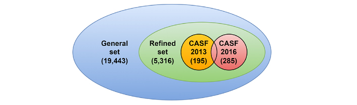
The PDBbind dataset and its components. The general set with 19,443 protein-ligand complexes, the refined set (included in the general) with 5,316 complexes, and both comparative assessment of scoring functions (CASF) benchmarks with 195 and 285 complexes respectively for the 2013 and the 2016 versions
In this work, the versions 2013 and 2016 of the core set are used as test sets (195 and 285 items, respectively), and 1,000 inputs from the refined set are randomly extracted to build the validation set and the remaining input as the training set (18,070 items). It is ensured that there are no duplicates between sets, except for the core sets which naturally have overlapping entries (elements from 2016 already present in the 2013 dataset). Also, in the pre-processing step, the protein files are cleaned by keeping only protein atoms, so that water and other hetero atoms are removed.
A graph
A heterogeneous graph, as presented in Figure 2, is composed of several graphs but in that case, only a pair of graphs, [
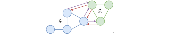
Example of a heterogeneous graph. Blue nodes belong to
Each molecule (protein and ligand) is represented with a graph of heavy atoms, thus, each graph node represents an atom, and the graph edges represent molecular bonds. A total of 23 physicochemical features are computed using Open Drug Discovery Toolkit (ODDT) [14] and are presented in Table 1. The 23 features are used as the second dimension for both the protein and ligand nodes. Then each ligand-protein atom pair closer than 4 Å is connected, also completed by a set of features enumerated in Table 2. Then after featurization is complete, each complex is represented by a protein graph
Nodes features
| Feature | Size | Description |
|---|---|---|
| Atom type | 8 | One-hot encoded (B, C, N, O, F, P, S, and others) |
| Hybridization | 7 | One-hot encoded (other, sp, sp2, sp3, sq planar, trigonal bipyramidal, octahedral) |
| Partial charge | 1 | Float (Gasteiger charge model) |
| Is hydrophobic | 1 | Boolean |
| Is in an aromatic cycle | 1 | Boolean |
| Is H-bond acceptor | 1 | Boolean |
| Is H-bond donor | 1 | Boolean |
| Is H-bond donor hydrogen | 1 | Boolean |
| Is negatively charged/chargeable | 1 | Boolean |
| Is positively charged/chargeable | 1 | Boolean |
Intra- and Inter-molecular edge features
| Feature | Size | Intra | Inter | Description |
|---|---|---|---|---|
| Length/distance | 1 | X | X | Float |
| Belongs to an aromatic cycle | 1 | X | - | Boolean |
| Belongs to a ring | 1 | X | - | Boolean |
| Type | 3 | X | - | One-hot (simple, double, or triple) |
| Is a hydrogen bond | 1 | - | X | Boolean |
| Is a salt bridge | 1 | - | X | Boolean |
| Is a hydrophobic contact | 1 | - | X | Boolean |
| Has π-stacking | 1 | - | X | Boolean |
| Has π-cation | 1 | - | X | Boolean |
π-stacking, and π-cation are only available for inter-molecular edges whose terminal atom from the protein side belongs to a ring. X: applicable; -: not applicable
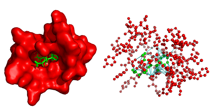
A protein-ligand complex and its associated heterogeneous graph. On the left, the 29G11 protein (in red) complexed with the ligand HEP in green (PDB: 1a0q). On the right, the heterogeneous graph represents the same complex, red nodes represent the protein binding site atoms, and the green nodes are the ligand atoms, both without hydrogen. Red and green edges represent intramolecular bonds, red edges belong to the protein while green edges belong to the ligand. Finally, the cyan edges are the inter-molecular links representing the protein-ligand interaction
Graph neural networks (GNNs) are a flexible type of neural objects that exist in various flavors, as classified by Wu et al. [15]. While recurrent GCNs (RGCNs) were the first attempt at modern graph neural modeling, nowadays GCNs are the most popular kind. GCNs are created by stacking multiple graph convolutional layers and updating the state of the graph at each step.
The implementation is based on PyTorch Geometric [16], a framework relying on the concept of message-passing neural network (MPNN, Equation 1) that includes libraries for sparse computation. Hence, the principle of spatial convolution as presented in Figure 4 is used.
Where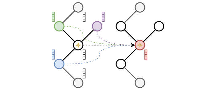
The spatial convolution process. In spatial convolution, the current node, here identified by a star, aggregates information coming from its direct neighbors here represented in green, purple, and blue. The current node feature vector is then updated as shown in the graph on the right
The proposed method is based on Attentive FP [17], which was adapted to work with molecular complexes. While the neural model was originally designed to produce a molecular fingerprint allowing the prediction of chemical properties such as toxicity or solubility, it was adapted to be applied to a molecular complex (ligand-protein) to produce a binding affinity score. That model is composed of graph attentional convolution (GATConv) and gated recurrent unit cell (GRUCell) layers, explained below.
The GATConv layer proposed by Veličković et al. [18] allows using an attention mechanism on GCN. In this work, the second version of the GATConv (GATv2Conv) layer proposed by Brody et al. [19] that fixes the static attention problem of GATConv is used. Thus, the network can learn which neighbor nodes are more relevant thanks to implicit weights. Indeed, in addition to the matrix of weights W, the GATConv operators learn an attention coefficient aij representing the magnitude of the edge j → i or in other words the importance of node features of j for explaining node i. All neighbors j of node i have a coefficient representing their importance for i. Equations 2 and 3 are used to compute the attention coefficient, and Equation 4 updates the current node features according to this coefficient.
Where the function e allows scoring the edge from j to i nodes, a and W are learned, the ‖ is the vector concatenation operator, ⊺ the transposition operator, and LeakyReLU the leaky rectified linear unit.As explained by Veličković et al. [18], all attention coefficients are normalized by a soft-max function over all node neighbors.
Where σ is a nonlinearity function.The GRUCell layer proposed by Cho et al. [20] is a recurrent neural network layer that keeps the memory of items over long sequences of data. A GRUCell layer is described by four equations to compute the layer update. The first two equations are the update gate (Equation 5) and the reset gate (Equation 6), respectively allowing relevant information to flow from the past (ht–1) or to be forgotten. The current memory content follows Equation 7 and stores the relevant information from the past. Finally, the layer is updated with Equation 8.
Where ⊙ is the Hadamard product.As mentioned above, the heterogeneous graph contains two sub-graphs (protein and ligand) in which nodes are connected. Thus, 4 types of edges: 𝒢p ↔ 𝒢p, 𝒢L ↔ 𝒢L, 𝒢p ↔ 𝒢L, and 𝒢L ↔ 𝒢p are used, resulting in 6 independent GCNs (one for each edge type in atomic part and one for each molecule in molecular part), and ending with a multi-layer perceptron (MLP) to compute the final score as presented in Figures 5–7. Different ways to construct the network including one that does not use the molecular embedding part and feeds the atomic embedding pooling to the MLP have been tested. The proposed method, used in the remainder of this paper, is the strategy that showed the best results.
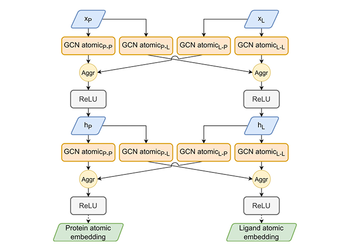
The HGScore atomic embedding part. The atomic embedding part extends Attentive FP atomic embedding to work on the heterogeneous graph to produce an atomic embedding of both molecules. The aggregation (Aggr) module allows a combination of previous layer outputs using mean, add, or max Aggr. ReLu: rectified linear unit
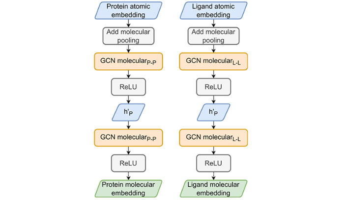
The HGScore molecular embedding part. The two atomic part embeddings are pooled by a sum to produce a molecular embedding which is used in the classical Attentive FP molecular embedding part to produce protein and ligand fingerprints

The HGScore prediction part. The two molecular part fingerprints are concatenated into an interaction fingerprint allowing an MLP to predict an affinity score
The atomic-GCN embedding part of the model, presented in Figure 5, encodes atomic features in a latent space. For both molecules, nodes are updated by two GCNs, one for each edge type. This resulted in four GCNs, all Attentive FP-inspired and using GATv2Conv and GRUCell. The main idea is to dissociate the embedding for each edge type so that each model will mix an intertwined pair of input signals enriched by their specific context (protein-protein, protein-ligand, ligand-protein, ligand-ligand). The resulting signal propagates information from context to context several times over by repeating the same operation.
Once the atomic-GCN embedding is completed, the same algorithm (Figure 6) proposed by Attentive FP (the molecular embedding) is applied to each molecule fingerprint, which consists of a sum global pooling, i.e., all node vectors are summed to produce a unique molecular representation. This vector is then processed by a molecular-GCN composed of GATv2Conv and GRUCell, also built from Attentive FP.
Finally, the concatenation of the two out-coming molecular fingerprints is used to produce the interaction fingerprint, which is fed to a classic feed-forward MLP (Figure 7), resulting in an affinity score of the complex.
To test and compare HGScore, the metrics and the two benchmarks (CASF 2013 and CASF 2016, also known as PDBbind core set 2013 and 2016) provided by Su et al. [13] are used. The Pearson correlation coefficient Rp (Equation 9) is used as the main metric, and the standard deviation (SD) in regression is the second (Equation 10). These metrics were proposed by Su et al. [13] as a good way to measure the scoring power of a scoring function. Rp allows determining if two sets of values are linearly correlated. Rp closer to 1.0 is considered best, with minimal SD. Other metrics of interest: the mean absolute error (MAE, Equation 11) and the root mean square error (RMSE) are also used (Equation 12).
Where xi is the predicted score for item i ∈ 〚1, n〛, yi the target score,Su et al. [13] also provide metrics to measure the ranking power of a scoring function; this power reflects the capacity of the function to correctly order a set of ligands docked on the same protein. Thus, Spearman’s rank correlation coefficient (ρ, Equation 13) [21], Kendall’s rank correlation coefficient (τ, Equation 14) [22], and the predictive index (PI) are used (Equation 15), all being within the interval [−1, 1] and 1 indicating a perfect ordering.
Where n is the number of ligands ranked for each target, it is 3 for CASF 2013 and 5 for the 2016 version, rxi is the rank of the predicted score xi, and ryi is the rank of the ground truth (obtained experimentally). PConcord and PDiscord correspond to the number of concording and discording pairs. Let a sample be a couple (xi, yi) with xi the predicted value and yi the ground truth, then a pair of sample [(xi, yi), (xj, yj)] is concording if xi < xj and yi < yj or xi > xj and yi > yj, is discording if xi < xj and yi > yj or xi > xj and yi < yj, else the pair is not counted.Where Wij = |yj − yi | andThe model is also assessed on the docking power [13] which allows to measure the capacity of a scoring function to detect near-native ligand binding poses among decoys. Two metrics are used, the first is the success rate in tops 1, 2, and 3 (the lowest predicted score is associated with the top 1 ligand, the second lowest to the top 2 ligand, and so on); then a given prediction is a success if the root mean square deviation (RMSD) (Equation 16) between the ligand in question and the native ligand pose is less than a cutoff value (2 Å). The second metric is the Spearman correlation coefficient (Equation 13) between the RMSD and the predicted score on different subsets of all ligands (decoys and native). The subset i contains all ligands whose RMSD (with the native one) is less than i, for i ∈ 〚2, 10〛.
Where P is the predicted atom coordinates, N is the native ligand atom coordinates, and n is the number of ligand atoms.The method’s implementation is based on PyTorch, Lightning, and PyTorch Geometric [16] to build the graph data, the datasets, and the model, and perform training and evaluation. Optuna was used to perform hyper-optimization to find the best architecture and perform the training with the same hyperparameter set several times over because the model is sensitive to weight initialization [23]. As a result, the model is composed of 3 atomic embedding layers with mean Aggr whose sizes are {48, 57, 68} for the protein part and {48, 76, 121} for the ligand part, followed by 4 molecular embedding layers. All atomic parts have 2 heads for their respective GATv2Convs. The interaction fingerprint is a vector of size 189 fed to an MLP with channels {189, 94, 1}.
During training, a learning rate of 10–3 associated with the Adam optimizer and a weight decay equal to 10−4 are used. The neural model is trained on 300 epochs with a dropout set at 0.13 (applied to all layers), but unpromising, stagnant candidates are stopped (with early stopping). The model was trained on an Nvidia DGX [a server with two sockets of 20 cores each, 512 gigabytes (GB) of random access memory (RAM)] using one graphics processing unit [GPU, an Nvidia V100 with 16 GB of video RAM (VRAM)], 300 epochs taking about 3 h00. The mean inference time is 0.10 s using one central processing unit (CPU), however, the necessary time to construct the graph from the complex file must be considered. That processing takes nearly 0.05 s (on the CASF 2016 complexes), but that time does not include the time for extracting the pocket if necessary, which is approximately 0.30 s per complex. The different times were not deeply studied because the other articles do not provide a basis for comparison. The results for the scoring power are presented in Figures 8 and 9 and Table 3. The scoring power results show a good Rp, especially for the CASF 2016, and both error metrics (MAE and RMSE) are pretty low, thus, the model is validated with respect to the scoring power.
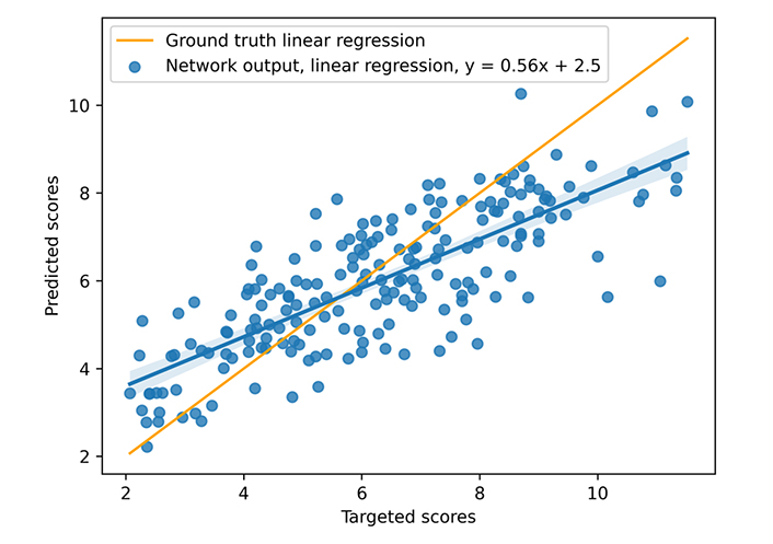
Results on CASF 2013. The blue points represent the predicted scores as a function of the targeted ones, the blue line is the blue points linear regression, and the orange line is the ground truth linear regression
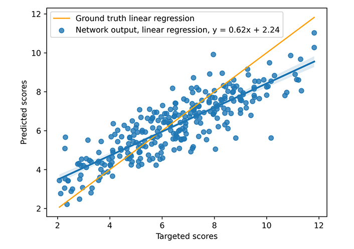
Results on CASF 2016. The blue points represent the predicted scores as a function of the targeted ones, the blue line is the blue points linear regression, and the orange line is the ground truth linear regression
Scoring power metrics for HGScore method on CASF 2013 and 2016
| Dataset | Rp | SD | MAE | RMSE |
|---|---|---|---|---|
| CASF 2013 | 0.79 | 1.39 | 1.11 | 1.39 |
| CASF 2016 | 0.85 | 1.14 | 0.90 | 1.14 |
↑ indicates that the larger the value, the better; ↓ indicates that the smaller the value, the better
Ranking power results are presented in Table 4, which shows that the model has good performance for the ranking power, especially on the CASF 2016 dataset.
Ranking power metrics for HGScore on CASF 2013 and 2016
| Dataset | PI | ||
|---|---|---|---|
| CASF 2013 | 0.59 | 0.55 | 0.60 |
| CASF 2016 | 0.74 | 0.67 | 0.76 |
↑ indicates that the larger the value, the better
Docking power results are presented in Tables 5 and 6. As shown in Table 5, the method ranks perfectly 1/3 of the native ligands (or a closer one) among the decoys. Moreover, the method ranks more than half of the native ligands (or a closer one) in the top 2 and 3. However, Table 6 does not show a good ranking performance; that lack of performance may be caused by the large number of used decoys and the small range of all scores (the average score range is 3.0) so the score range being small the model has more chance of not respecting the RMSD ranking. It should be noted that the fact that the produced scores are in a small range is because all the experimental scores of the training set are themselves in a small range.
The docking power success rate (%) on the CASF 2016 dataset
| TOP 1 | TOP 2 | TOP 3 |
|---|---|---|
| 32.63 | 51.93 | 60.35 |
The docking power Spearman correlation coefficient metric on CASF 2016
| RMSD range( | Coefficient |
|---|---|
| [0, 2] | 0.17 |
| [0, 3] | 0.20 |
| [0, 4] | 0.23 |
| [0, 5] | 0.25 |
| [0, 6] | 0.26 |
| [0, 7] | 0.27 |
| [0, 8] | 0.28 |
| [0, 9] | 0.30 |
| [0, 10] | 0.30 |
↑ indicates that the larger the value, the better
In addition to the intrinsic characterization of the new scoring method, the HGScore results are compared to some other DL scoring methods in Tables 7 and 8 respectively for CASF 2013 and 2016. The other methods compared are Pafnucy [4], DeepBindRG [5], OnionNet [7], IGN [10], and ECIF6::LD-GBT [11]. Some classical scoring function performances on CASF 2013 [24] and CASF 2016 [13] are presented to provide a no AI-centric comparison.
Metrics computed on the CASF 2013
| Method | Trained on PDBbind | N | Rp | SD | MAE | RMSE |
|---|---|---|---|---|---|---|
| GoldScore | - | 195 | 0.48 | 1.97 | - | - |
| ChemScore | - | 195 | 0.59 | 1.82 | - | - |
| X-ScoreHM [24] | - | 195 | 0.61 | 1.78 | - | - |
| DeepBindRG [5] | 2018 | 195 | 0.64 | - | 1.48 | 1.82 |
| Pafnucy [4] | 2016 | 195 | 0.70 | 1.61 | - | 1.62 |
| OnionNet [7] | 2016 | 108 | 0.78 | 1.45 | 1.21 | 1.50 |
| AGL-Score | 2007 (refined) | 195 | 0.79 | - | - | 1.97 |
| IGN | 2016 | 85 | 0.83 | - | - | - |
| HGScore | 2016 | 195 | 0.79 | 1.39 | 1.11 | 1.39 |
The scoring function was used with the software a Gold and b Sybyl. c the number of tested complexes is too low to be compared with the other methods. ↑ indicates that the larger the value, the better; ↓ indicates that the smaller the value, the better. N is the number of tested complexes, some methods have been tested only on a subset of the benchmark. -: not applicable
Metrics computed on the CASF 2016
| Method | Trained on PDBbind | N | Rp | SD | MAE | RMSE |
|---|---|---|---|---|---|---|
| GoldScore | - | 285 | 0.42 | 1.99 | - | - |
| ChemScore | - | 285 | 0.59 | 1.76 | - | - |
| X-ScoreHM [13] | - | 285 | 0.61 | 1.73 | - | - |
| Pafnucy [4] | 2016 | 290 | 0.78 | 1.37 | 1.13 | 1.42 |
| Pafnucy | 2020 | 285 | 0.76 | - | - | 1.46 |
| OnionNet [7] | 2016 | 290 | 0.82 | 1.26 | 0.98 | 1.28 |
| AGL-Score | 2007 (refined) | 285 | 0.83 | - | - | 1.73 |
| IGN [10] | 2016 | 262 | 0.84 | - | 0.94 | 1.22 |
| ECIF6::LD-GBT | 2016 (refined) | 285 | 0.87 | - | - | - |
| HGScore | - | 285 | 0.85 | 1.14 | 0.90 | 1.14 |
The scoring function was used with the software a Gold and b Sybyl. c a problem for comparison, either the dataset is not fully tested, or the test set is also used for training or validation. ↑ indicates that the larger the value, the better; ↓ indicates that the smaller the value, the better. N is the number of tested complexes, some methods have been tested only on a subset of the benchmark, methods with N of 290 have been tested on a former CASF 2016 version. -: not applicable; *: retrained on the same split as HGScore
HGScore is among the best results on the CASF datasets for the scoring power metrics (Table 8), and the ability of the method to split the learning following the bond type may be an important part of the improvement. However, compared to existing scoring methods, the proposed new score does not bring significant improvement in the case of the CASF 2013 dataset (Table 7); it may be because the model of the present study has been trained on PDBbind version 2020. Indeed, the CASF datasets are the most representative complexes of PDBbind respectively in versions 2013 and 2016. Although the IGN method has a Rp of 0.83, the CASF 2013 test set is reduced to only 85 items which is far from the whole set, thus it is difficult to conclude about this Rp value. Concerning the ECIF6::LD-GBT method, the CASF 2016 is used for both the validation and test sets, whereas for HGScore the test set is unknown when the model is tested on it, which is the canonical way of proceeding. On the other hand, some authors have trained their method on the PDBbind refined set, which is composed of the highest quality complexes, but that choice may imply a lower prediction quality on the poorest quality complexes, which are the most frequent ones. It also should be noted that some methods do not provide any other metric than Rp, involving a greater difficulty in comparison.
The IGN method is the one that most resembles HGScore, indeed, the HGScore heterogeneous graphs can be considered as the assembly of the three independent graphs of the IGN method.
The present model has been trained on the 2020 version of PDBbind. The 2016 version of CASF is closer in terms of composition, which explains why HGScore improves the performance on the latter but not on the 2013 version. Nevertheless, it should be noted that on the CASF 2013, HGScore outperforms the others since it leads to lower error metrics values: the MAE and the RMSE.
Since the training set impacts the results of the scoring, it is of utmost importance to compare the performance of the HGScore with the performance of the score of other methods trained, validated, and tested identically. That is why the Pafnucy method [4] was also trained from scratch on the same HGScore dataset split. Tested on CASF 2016 (Table 8), the HGScore method still outperforms Pafnucy trained in a completely identical way (starred line in Table 8). Because of the difficulty to get the source codes and then to execute them easily, in a strictly identical way to HGScore, only the Pafnucy method has been retrained.
In conclusion, the new proposed DL method allows scoring protein-ligand complexes. Based on the Attentive FP method, the presented model brings the originality to split the learning process regarding the interaction class, ligand to ligand, protein to protein, ligand to protein, and protein to ligand. That general idea allows the model to learn more precisely the effect of the molecules themselves and the interaction between them. The method does not propose a new type of layer but rather a new way to represent ligand-protein complexes, using a heterogeneous graph. Trained on the PDBbind dataset, like almost all counterpart methods, HGScore reaches the top of the methods assessed on the CASF 2016 dataset. Moreover, the method largely outperforms the classical scoring methods presented in a previous article [1]. Although HGScore does not bring a huge improvement on the main test metric (Rp on CASF 2016), it outperforms all methods blindly tested on CASF. Moreover, the quality already achieved by the metrics implies that their improvement cannot be very large anymore.
As mentioned previously the network is split according to the interaction category. This method will allow to easily use transfer learning and thus reuse the feature extractor and high-level abstract representation based on the type of interaction between the two molecular groups. Of course, it will be necessary to ensure that the roles of the receptor (here the protein) and the ligand are preserved. Therefore, the use of transfer learning to adapt this new model to cases of protein-glycosaminoglycan (GAG) or protein-proteoglycan docking is very promising.
The next objective will be to integrate that scoring function into a complete docking process and analyze a) its impact on docking results and understand the root cause for better performance over other docking programs such as AutoDock and b) its impact on computation time. For now, HGScore can be used as an external scoring function allowing to reassess the score of a set of docked complexes to refine existing ranking.
3D: three-dimensional
Aggr: aggregation
AGL-Score: algebraic graph learning score
AI: artificial intelligence
CASF: comparative assessment of scoring functions
DL: deep learning
GATConv: graph attentional convolution
GATv2Conv: graph attentional convolution version 2
GCNs: graph convolutional networks
GNNs: graph neural networks
GRUCell: gated recurrent unit cell
HGCN: heterogeneous graph convolutional network
HGScore: heterogeneous graph score
IGN: InteractionGraphNet
MAE: mean absolute error
ML: machine learning
MLP: multi-layer perceptron
PDB: Protein Data Bank
PDBbind: Protein Data Bank-bind
RMSD: root mean square deviation
RMSE: root mean square error
SD: standard deviation
The authors thank the supercomputer center ROMEO for providing CPU-GPU times.
KC: Conceptualization, Software, Writing—original draft, Writing—review & editing. AG: Software, Writing— review & editing, Supervision. XV, SB, and LAS: Writing—review & editing, Supervision. All authors read and approved the submitted version.
The authors declare that they have no conflicts of interest.
Not applicable.
Not applicable.
Not applicable.
The datasets analyzed for this study can be found in the PDBbind website http://pdbbind.org.cn/.
This work was supported by the Association Nationale de la Recherche et de la Technologie (ANRT) through a CIFRE grant [2020/0691]. The funders had no role in study design, data collection and analysis, decision to publish, or preparation of the manuscript.
© The Author(s) 2023.
Copyright: © The Author(s) 2023. This is an Open Access article licensed under a Creative Commons Attribution 4.0 International License (https://creativecommons.org/licenses/by/4.0/), which permits unrestricted use, sharing, adaptation, distribution and reproduction in any medium or format, for any purpose, even commercially, as long as you give appropriate credit to the original author(s) and the source, provide a link to the Creative Commons license, and indicate if changes were made.

Walter F. de Azevedo Jr.
Minyi Su, Enric Herrero
