Original Article

Affiliation:
1Department of Statistics, Duksung Women’s University, Seoul 01369, Republic of Korea
ORCID: https://orcid.org/0009-0001-9856-786X
Affiliation:
2Department of Brain and Cognitive Sciences, Seoul National University, Seoul 03080, Republic of Korea
ORCID: https://orcid.org/0000-0003-3485-2327
Affiliation:
1Department of Statistics, Duksung Women’s University, Seoul 01369, Republic of Korea
Email: jaehee@duksung.ac.kr
ORCID: https://orcid.org/0000-0002-2115-0142
Explor Neuroprot Ther. 2023;3:446–456 DOI: https://doi.org/10.37349/ent.2023.00061
Received: June 27, 2023 Accepted: September 25, 2023 Published: December 13, 2023
Academic Editor: Valery V. Tuchin, Saratov State University, Russia
Aim: Recently, brain network research is actively conducted through the application of graph theory. However, comparison between brain networks is subject to bias issues due to topological characteristics and heterogeneity across subjects. The minimum spanning tree (MST) is a method that is increasingly applied to overcome the thresholding problem. In this study, the aim is to use the MST analysis in comparing epilepsy patients and controls to find the differences between groups.
Methods: The MST combines entities for epileptic magnetoencephalography (MEG) data. The MST was applied and compared to 21 left surgery (LT) and 21 right surgery (RT) patients with epilepsy and good postoperative prognosis and a healthy control (HC) group. MST metrics such as betweenness centrality, eccentricity, diameter, and leaf fraction, are computed and compared to describe the integration and efficiency of the network. The MST analysis is applied to each subject, and then the integrated MST is obtained using the distance concept. This approach can be advantageous when comparing the topological structure of patients to controls with the same number of nodes.
Results: The HC group showed less topological change and more network efficiency than the epilepsy LT and RT groups. In addition, the posterior cingulate gyrus was found as a hub node only in the patient group in individual and integrated subject data analysis.
Conclusions: This study suggests propose that the hippocampus borrows from the default network when one side fails, compensating for the weakened function.
The minimum spanning tree (MST) method is a helpful tool that avoids some problems arising in brain network analysis [1, 2]. The MST analysis can provide insights into how the brain processes information and how different regions work together to support cognitive functions [3, 4]. By analyzing the MST of a functional brain network, researchers can identify the most efficient communication pathways between different brains [1, 3].
MST is insensitive to link strength or density changes and is equally sensitive to network topology changes as in conventional graph theory measurements. Therefore, it is convenient for comparative studies between brain networks [3].
In graph theory, a tree is defined as a connected graph without the formation of any loops. Employing MST is a solution to comparing network topologies under different conditions since there is no need to set thresholds and use a fixed number of nodes and edges. The MST method has the advantage that the MST of the weighted linkage metric is unique when the weights are unique [1]. Although many connections are removed due to the nature of this method, it is equally sensitive to the network topology as the existing graph theoretical measurement [2]. The potential of brain network properties to serve as neurological and psychopathological biomarkers is hampered by threshold problems. The MST is free from this problem, so it has increasingly been applied [1].
The MST metric is also robust against substantial noise in the data [5]. It is actively used in brain research related to brain diseases, and there are various MST-based research results related to this area.
In MST studies [5], MST leaf area significantly correlates with the network size, although MST analysis has not yet led to definitive neuropsychiatric symptoms or disease biomarkers.
Studies investigating Alzheimer’s disease (AD), a neurodegenerative disorder, using MST analysis by analyzing the functional connectivity, examined differences in brain networks between AD patients and healthy controls (HCs). The AD group showed a less integrated structural network with such MST metrics as a higher characteristic path length, but lower leaf fraction [6].
An abnormal MST structure is observed in patients with AD and mild cognitive impairment (MCI). In a study [7–9] using resting functional magnetic resonance imaging (fMRI) to examine functional brain connectivity changes in AD and MCI patients, AD and MCI patients showed abnormal MST characteristics in functional brain networks related to cognitive performance.
Over time, changes in MST properties in AD patients correlate with disease progression [7–9]. The MSTs for classifying Parkinson’s disease and essential tremor patients from diffusion magnetic resonance imaging (dMRI) data study use dMRI to investigate the brain’s structural connectivity. This result demonstrated differences in brain network connectivity between Parkinson’s disease and essential tremor patients [10].
MST analysis of the human connectome is employed to investigate the structural connectivity of the human brain. The study [11] examined various characteristics of the human brain’s connectivity (e.g., connection strength and type) using MST analysis and revealed that specific brain regions are more strongly connected to other brain regions.
MST methods are related to the severity of Parkinsonian cognitive impairment to neural connectivity changes [12]. Yan et al. (2019) used MST analysis to investigate changes in the global topology of functional brain networks and explore the relationship between these changes and cognitive function [13].
The study aims to investigate the difference in the global topology of brain networks in epilepsy patients via MST analysis. The epilepsy patients had an altered MST compared to HCs, with longer path lengths and decreased clustering coefficients. The degree of MST alteration was associated with the frequency and duration of seizures [14].
In this paper, individual and group-wise MST analyses are conducted for epilepsy patients and HCs. The main goal of this study is to examine whether there are any changes in the overall topology of brain networks among individuals and groups with epilepsy by employing MST analysis. Additionally, the aim to investigate the relationship between these alterations in network structure and specific epilepsy-related characteristics. The MST metrics are also computed for the resulting MSTs for group comparison.
Data are from patients with histopathologically proven hippocampal sclerosis (HS) and postoperative seizure-free medial temporal lobe epilepsy (mTLE) who underwent epilepsy surgery at Seoul National University Hospital between 2005 and 2011. Data from 46 healthy subjects and 44 patients (left mTLE = 22; right mTLE = 22) were analyzed. The HC group comprised 19 males and 27 females, with a mean age of 29. Also, the mTLE consisted of 10 males and 12 females (left), seven males and 15 females (right), with mean ages of 31 (left) and 32 (right).
Amygdalohippocampectomy (left mTLE consists of 10 patients and right mTLE has 14 patients) or selective amygdalohippocampectomy (left mTLE consists of 12 patients and right mTLE has 8) patients for anterior temporal lobectomy.
One left surgery (LT) patient and one right surgery (RT) patient were excluded from this study since the number of time-points measured is less than 20,000. Therefore, the total number of analyzed subjects was 86, with 21 in the LT group, 21 in the RT group, and 46 in the HC group.
Magnetoencephalography (MEG) recordings were made in a 306-channel, whole-head system (Vectorview, Elekta Neuromag Oy, Finland). The predefined 72 nodes (36 nodes in each hemisphere) are involved with a set of 2 central, 12 frontal, 4 temporal, 5 parietal, 7 occipital, and 6 limbic regions in each hemisphere. These region of interest (ROI) nodes were selected from the automated anatomic labeling (AAL) atlas. The MEG sensors were arranged at locations where triplets consisting of two orthogonal planar gradiometers and one magnetometer were included. Recordings were obtained and formed at a sampling frequency of 600.615 Hz inside the magnetically shielded room. Electrooculography and electrocardiography data were recorded simultaneously. Data were collected during the 15-minute epoch while mTLE patients were lying supine with their eyes closed.
For HC, two minutes of MEG data were recorded during a resting-state eyes-closed and eyes-open condition when sitting or lying supine. MEG data consists of a brain network in which each ROI becomes a node, and a connection between the two nodes becomes a link. Each subject MEG data is obtained from time-points 1 to 30,000 with the time interval as 10,000 points.
A spanning tree is a graph of the least-connected parts of a graph, where the slightest connection means the least number of links. The minimum number of edges in a graph with N vertices (nodes) is N–1. If N–1 edges connect them, it inevitably becomes a tree called a spanning tree. There can be many spanning trees in one graph.
A spanning tree is a particular type of tree, so all vertices must be connected and not contain cycles. Among the spanning trees, the tree with the smallest sum of used link weights is the MST.
MST is the edge weight of an undirected graph and a subset of connected edges connecting all vertices with the most negligible possible total edge weight without recursion. MST stands for the minimum cost spanning tree, considering the weights on the edges. That is, it connects all vertices on the network with weights assigned to the links with the fewest links and cost.
Considering the weights of edges, a minimum cost spanning tree connects all vertices in the network with weights assigned to the link with the least number of links and the least cost. There can be multiple minimum-spanning trees with equal weights. If all link weights in a given graph are equal, all spanning trees are minimal. If each link has its weight, there is only one unique MST.
MEG data is a network obtained by measurement according to time-points and is a time-varying network structure. MEG’s dynamic functional connectivity (DFC) is measured over time to form a temporal network. A temporal network graph is expressed as follows, including a set D along the time-point dimension:
Eqn. 2.1:
where V is a set containing N nodes, and E is a set of tuples that are the edges or connections between pairs of nodes.
Degree is defined as the number of links for a given node that measure regional importance with aij in the adjacent matrix in (2.2) as
Eqn. 2.2:
MST measurements are briefly introduced [5, 11, 15]. MST measures represent the integration and efficiency of the network such as diameter, leaf fraction, betweenness centrality (BC), and tree hierarchies. A network with a small diameter and a high leaf fraction is a centralized network, and a network with a high diameter and a low leaf fraction is a non-centralized network [16]. The diameter is the longest distance between any two nodes within the network and represents integrity and efficiency. The normalization of the diameter is expressed as
Eqn. 2.3:
where d is the diameter and M is the total number of links or the maximum number of leaves M = N –1.
A measure of centrality can be made based on the number of leaves. The leaf fraction Lf is the number of leaves where L is the number of nodes with only one connection divided by the maximum number of leaves M such as
Eqn. 2.4:
The lower the value of the leaf ratio, the less centralized the network topology, and the higher the leaf ratio, the more the network depends on the hub node for communication. The leaf fraction decreases as the network size increases [16]. The higher the leaf fraction, the more integrated the network [17]. BC measures the importance of a node in the network, defined as:
Eqn. 2.5:
where σij is the total number of shortest paths from node i to j and σij (v) is the number of those paths that pass through v. The node with the highest BC has the highest number of shortest paths between two nodes through it [5, 15]. BC measures the fraction of the shortest paths passing through a node. A node with a high BC value suggests that the node is playing a bridge-spanning role [5, 15, 17].
MST and statistical analyses were performed in R (version 4.3.1) using packages igraph and network, and custom R functions.
The following steps were applied for the analysis of epilepsy MEG data. In this study, epilepsy patients and HCs underwent MEG, neuropsychological assessment, and neurological examination. MST metrics were utilized for the analysis of variance (ANOVA) for group comparison.
The MEG data at the sensor level were projected onto an AAL atlas using beamforming, resulting in a 72-time series for each ROI (Figure 1A). The correlation coefficients between pairs of ROIs based on the entire time were calculated. A 72 × 72 adjacency matrix is constructed. This adjacency matrix is reconstructed based on the hierarchical clustering and shown in the image plot (Figure 1B). Considering the concept of distance with pairwise Pearson correlation r, calculate d = 1 – |r| for the adjacency matrix. Then the Prim algorithm was applied to obtain the MST matrix (Figure 1C). This distance was chosen as the simplest way to minimize bias in converting to the distance concept from correlation. The data is divided into three accumulated parts for the analysis according to three time-points. Optionally, three time-points at 10,000 (T1), 20,000 (T2), and 30,000 (T3) are chosen.
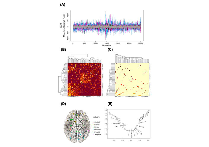
Overview of the applied methods (lt020 patient for example). (A) MEG data; (B) connectivity image plot reordered with hierarchical clustering; (C) connectivity image plot reordered with MST analysis; (D) network graph with MST result; (E) tree graph with MST result on two first nsca axes
The MST analysis pipeline is illustrated in Figure 1. This MST is displayed as a graph on a brain image (Figure 1D). An example of a weighted MST tree graph is shown in Figure 1E. The overlapped nodes in Figure 1E are indicated as close to each other. The axes are the two first non-symmetric correspondence analyses (nsca, [18, 19]). The two dimensions of nsca are determined through principal component analysis (PCA) to maximize the variability in the original data along these two centered axes. The tree structure in Figure 1E is listed with the linked nodes as follows:
1-36, 2-22, 2-32, 2-42, 2-43, 2-59, 3-7, 3-11, 3-52, 4-34, 5-15, 5-32, 6-13, 6-32, 7-47, 8-31, 8-38, 8-44, 8-45, 8-57, 9-45, 10-14, 10-33, 10-71, 11-50, 12-46, 14-69, 16-21, 16-32, 17-35, 18-30, 18-32, 19-25, 20-24, 23-35, 23-60, 24-59, 25-26, 26-65, 27-29, 28-63, 29-61, 30-66, 31-33, 31-36, 31-41, 32-62, 33-39, 33-46, 34-70, 35-67, 35-71, 36-54, 36-63, 37-58, 40-48, 43-50, 48-50, 49-69, 51-53, 51-65, 51-66, 52-58, 55-57, 56-60, 61-72, 63-65, 64-65, 67-68, 67-70, 71-72.
Integrating individual data into one representative is a complicated problem, especially in combining the MEG data in each group. The researchers have yet to find the suggested way to combine MST from the previous research. Therefore, a new solution was tried in this article. Each MST was derived from the individual MEG network. Then an integrated MST was made by combining these MSTs with some weight matrices. The suggested steps are as follows. Here the connectivity measure should be converted to the distance measure.
First, the MST for each subject is obtained, followed by the application of the distance concept at a given time-point. Second, each subject MST matrix Ti is component-wise multiplied by each subject weight matrix wi for MST Ti, resulting in integrated MST. Here Ng is the generative total number of group g. As a distance metric for MST. The following matrix computed as a distance metric for MST within each group.
Eqn. 2.6:
Here ° is an element-wise product operator known as Hadamard product. Individual weight matrix wi is defined as the degree of each node of an individual MST Ti.
Subtraction is made to make the distance for the MST. Finally, the resulting model is created by applying MST to ITg such as
Eqn. 2.7:
The integrated MST model can be a representative MST in each group at the corresponding time.
Hub nodes in each subject MST were initially identified. In each group, the hub node was defined as a hub node when it was not only selected as the hub node from individual data but also as the hub node from more than five subjects. Then, the top three hub nodes were selected.
One important finding is that hub node 71 [posterior cingulate gyrus, limbic(right)] appears only in the patient LT and RT. Nodes 10 (superior frontal gyrus, orbital part) and 11 (superior frontal gyrus, medial orbital) in the orbital surface area were found as hub nodes at whole time-points of LT and HC. Node 33 (anterior cingulate and paracingulate gyri), corresponding to the limbic system, was selected as a hub node (an average of 12 times) throughout the whole time-points in HC. The hub nodes in each group by time-point are briefly summarized in Table 1.
Hub nodes of MSTs by group at time-point T1 = 10,000, T2 = 20,000, T3 = 30,000
| Group | Hub node | ||
|---|---|---|---|
| Time | |||
| T1 | T2 | T3 | |
| LT | 10, 32, 71 | 10, 32, 71 | 10, 32, 71 |
| RT | 10 | 10, 11, 71 | 10, 32, 71 |
| HC | 3, 32, 33 | 3, 32, 33 | 3, 32, 33 |
Additionally, MST metrics were calculated and mean comparisons were performed using ANOVA and Kruskal-Wallis tests with nonnormality at each time-point. There was no significant difference between groups in a maximum BC but significant in means of BC. The average shortest path length in HC is also the lowest. Significant differences were observed at each time-points.
The eccentricity shows a significant difference only at time-point T2. Moreover, RT had the highest eccentricity. As a result of Tukey’s post-hoc analysis on eccentricity at time-point T2, one group (HC, LT) with RT was determined as one group.
The diameter was the largest in RT, but no statistically significant difference was found. The diameter and eccentricity of LT fluctuated between time-points. Further investigation is required in these measures.
The leaf fraction showed a significant difference at the T1 time-point. The leaf fraction was high in patients with epilepsy. Also, there was no significant difference between T2 and T3 time-points. In the whole time-points, RT has the most considerable eccentricity, diameter, and the average shortest path length. It tells that the RT patient network efficiency is the worst among the three groups.
Our data showed no significant difference between the tree hierarchy overlaps in seizure-free epileptic patients with an excellent postoperative prognosis. It supports the results of previous studies [16, 20]. The MST metrics summary and ANOVA results are shown in Table 2.
MST metrics and mean comparison test results by group at time-point T1 = 10,000, T2 = 20,000, and T3 = 30,000
| Metrics | Time | Group | Statistic | P-value | ||||
|---|---|---|---|---|---|---|---|---|
| LT | RT | HC | AOV | Kruskal-Wallis | AOV | Kruskal-Wallis | ||
| Max of degree | T1 | 6.381 (1.203) | 5.571 (0.978) | 6.174 (1.141) | 3.083 | 5.540 | 0.051 | 0.063 |
| T2 | 6.429 (1.165) | 5.905 (1.091) | 6.065 (1.000) | 1.379 | 2.308 | 0.257 | 0.315 | |
| T3 | 6.476 (1.436) | 5.762 (1.044) | 6.109 (1.100) | 1.939 | 3.606 | 0.150 | 0.165 | |
| Max of BC | T1 | 0.627 (0.044) | 0.648 (0.043) | 0.632 (0.050) | 1.172 | 3.168 | 0.315 | 0.205 |
| T2 | 0.648 (0.055) | 0.648 (0.054) | 0.635 (0.051) | 0.613 | 1.082 | 0.544 | 0.582 | |
| T3 | 0.636 (0.047) | 0.631 (0.042) | 0.640 (0.054) | 0.187 | 0.217 | 0.830 | 0.897 | |
| Mean of BC | T1 | 0.098 (0.010) | 0.102 (0.011) | 0.095 (0.009) | 4.620 | 7.901 | 0.012* | 0.019* |
| T2 | 0.093 (0.009) | 0.102 (0.013) | 0.095 (0.008) | 5.183 | 6.469 | 0.008* | 0.040* | |
| T3 | 0.101 (0.012) | 0.100 (0.010) | 0.095 (0.009) | 3.449 | 7.902 | 0.036* | 0.019* | |
| Eccentricity | T1 | 14.612 (1.637) | 15.183 (2.075) | 14.304 (1.788) | 1.670 | 3.181 | 0.194 | 0.204 |
| T2 | 13.928 (1.446) | 15.126 (1.939) | 14.261 (1.551) | 3.139 | 5.224 | 0.048* | 0.073 | |
| T3 | 15.033 (1.928) | 15.085 (1.567) | 14.280 (1.755) | 2.166 | 5.843 | 0.121 | 0.054 | |
| Diameter | T1 | 18.620 (2.224) | 19.524 (2.909) | 18.478 (2.492) | 1.267 | 2.634 | 0.287 | 0.268 |
| T2 | 17.857 (1.852) | 19.571 (2.461) | 18.413 (2.146) | 3.518 | 5.923 | 0.034* | 0.052 | |
| T3 | 19.095 (2.385) | 19.619 (2.012) | 18.522 (2.483) | 1.638 | 4.889 | 0.200 | 0.087 | |
| Average shortest path length | T1 | 7.883 (0.690) | 8.160 (0.780) | 7.620 (0.637) | 4.620 | 7.901 | 0.012* | 0.019* |
| T2 | 7.541 (0.648) | 8.149 (0.893) | 7.646 (0.571) | 5.183 | 6.469 | 0.008* | 0.039* | |
| T3 | 8.058 (0.857) | 7.991 (0.703) | 7.619 (0.675) | 3.449 | 7.902 | 0.036* | 0.019* | |
| Tree hierarchy | T1 | 0.011 (0.001) | 0.011 (0.001) | 0.011 (0.001) | 1.343 | 3.168 | 0.267 | 0.205 |
| T2 | 0.011 (0.001) | 0.011 (0.001) | 0.011 (0.001) | 0.630 | 1.082 | 0.535 | 0.582 | |
| T3 | 0.011 (0.001) | 0.011 (0.001) | 0.011 (0.001) | 0.127 | 0.217 | 0.881 | 0.897 | |
| Leaf fraction | T1 | 0.450 (0.041) | 0.418 (0.048) | 0.454 (0.038) | 5.795 | 8.639 | 0.004* | 0.013* |
| T2 | 0.451 (0.036) | 0.427 (0.041) | 0.449 (0.038) | 2.883 | 4.743 | 0.061 | 0.093 | |
| T3 | 0.449 (0.029) | 0.427 (0.043) | 0.444 (0.039) | 2.024 | 3.370 | 0.139 | 0.186 | |
* means statistically significant at 0.05 level; ANOVA is denoted as AOV
As discussed earlier, the MST method might be precious when comparing patients with controls. Because MST networks have a unique advantage that does not need a threshold, and MST networks from different groups contain the same number of nodes and connections. The MST metric results, which integrate individual data into one, were measured at 30,000 time-points.
What is noteworthy in this study is that node 71 was designated as a hub node only in the patient group in the integrated data as well as in the individual data analysis.
In addition, as a result of checking the centrality values of the 71st node, the LT group had 0.391, RT 0.389, and HC 0.028, which showed higher centrality of mediation in the patient group.
Similar to the individual data analysis, RT had the highest degree, and there was no significant difference between the control and patient groups in leaf fraction or tree hierarchy. On the other hand, in the integrated data, the LT group showed the highest BC and average shortest path length. However, the HC group still appears to have the best network efficiency with the smallest eccentricity, BC, average shortest path length, and diameter. The summarized results are presented in Table 3.
Results of MST integrated by group
| Metrics/group | LT | RT | HC |
|---|---|---|---|
| Hub node (degree ≥ 5) | 71, 10, 32, 2 | 11, 71, 10, 8 | 11, 32, 33, 3 |
| Max of degree | 6 | 8 | 7 |
| Max of BC | 0.594 | 0.667 | 0.627 |
| Mean of BC | 0.110 | 0.091 | 0.079 |
| Eccentricity | 16.236 | 13.097 | 11.667 |
| Diameter | 20 | 17 | 15 |
| Average shortest path length | 8.709 | 7.394 | 6.524 |
| Tree hierarchy | 0.841 | 0.750 | 0.798 |
| Leaf fraction | 0.521 | 0.479 | 0.479 |
Integrated with weights was performed to draw an MST on the brain image in each group. In Figure 2, node 71 (the posterior cingulate gyrus) stands out in the LT and RT groups at the lower 2/3 part of the brain in the middle.
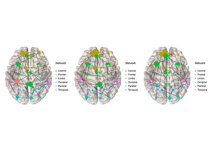
Integrated MST at time-point = 30, 000 (T3) for LT (left), RT (middle), and HC (right)
Our results show that the results of the RT group in individual metrics are less likely to have a network effect. It is unknown whether these results are related to the surgical operation, and it is unlikely that this is a characteristic of patients who underwent surgery on the right side. However, it was found that HC had a shorter average shortest path length and average mediation centrality for both LT and RT groups.
The posterior cingulate gyrus in the patient group is known as the default network of the hippocampus in the limbic system. Our results show that only in the patient group, node 71, this default network is continuously active as the hub node, in contrast to the control group. It can hint that the default network is activated in the patient group. Our results suggest that, in the end, when one side of the hippocampus breaks down, it borrows from the default network to compensate for the weakened function. In addition, our patients had good prognosis because the surgery went well. Nevertheless, there were differences in topology and hub nodes between groups. At each time-point, our integrating method can be considered to combine and summarize the subject MSTs in each group.
The MST with MEG data for epileptic patients and HC group was analyzed. The MST analysis is adopted to compare these groups because it facilitates topological information with fixed edges. There are few previous MST merging studies for brain imaging data. Our study suggests aggregating the individual MST results with node degree. Rather than applying MST to simple average connectivity, our method combines individual MSTs with node degree weights. This method can incorporate the individual MST information and degree information together. MST metrics can distinguish the patient and control groups. Our method can be used as topological features in individual and integrated ways.
AD: Alzheimer’s disease
BC: betweenness centrality
HC: healthy control
LT: left surgery
MCI: mild cognitive impairment
MEG: magnetoencephalography
MST: minimum spanning tree
mTLE: medial temporal lobe epilepsy
nsca: non-symmetric correspondence analyses
ROI: region of interest
RT: right surgery
SS: Conceptualization, Formal analysis, Investigation, Methodology, Project administration, Software, Validation, Writing—original draft, Writing—review & editing. CKC: Conceptualization, Data curation, Resources, Writing—review & editing. JK: Conceptualization, Funding acquisition, Project administration, Validation, Writing—review & editing, Supervision. All authors read and approved the submitted version.
The authors declare that they have no conflicts of interest.
The study protocol was approved by the Seoul National University Hospital Institutional Review Board (IRBH-0607-029-178).
Informed consent to participate in the study was obtained from all participants.
Not applicable.
The datasets for this manuscript are not publicly available because raw data were generated at Seoul National University Hospital. Requests for accessing the datasets should be directed to Dr. Chung (chungc@snu.ac.kr).
This work was supported by the National Research Foundation of Korea (NRF) grant funded by the Korea government (MSIT) [No. 2021R1A4A5028907] and Basic Research [No. 2021R1F1A1054968]. The funders had no role in study design, data collection and analysis, decision to publish, or preparation of the manuscript.
© The Author(s) 2023.
Copyright: © The Author(s) 2023. This is an Open Access article licensed under a Creative Commons Attribution 4.0 International License (https://creativecommons.org/licenses/by/4.0/), which permits unrestricted use, sharing, adaptation, distribution and reproduction in any medium or format, for any purpose, even commercially, as long as you give appropriate credit to the original author(s) and the source, provide a link to the Creative Commons license, and indicate if changes were made.