 Original Article

Affiliation:
V.B. Sochava Institute of Geography, Siberian Branch of the Russian Academy of Sciences, 664033 Irkutsk, Russian Federation
ORCID: https://orcid.org/0000-0002-7596-7780
Affiliation:
V.B. Sochava Institute of Geography, Siberian Branch of the Russian Academy of Sciences, 664033 Irkutsk, Russian Federation
Email: knesun@mail.ru
ORCID: https://orcid.org/0000-0001-7643-6693
Explor Digit Health Technol. 2025;3:101168 DOI: https://doi.org/10.37349/edht.2025.101168
Received: December 14, 2024 Accepted: August 28, 2025 Published: October 29, 2025
Academic Editor: Sil Aarts, Maastricht University, Netherlands; Atanas G. Atanasov, Medical University of Vienna, Austria
The article belongs to the special issue Data-informed Decision Making in Healthcare
Aim: This study analyses the time series of daily increases in the number of diagnosed COVID-19 cases in Russia and countries from different continents. The aim of the study is to identify the specifics of the population response of different countries to the spread of the pandemic and anti-epidemic measures of public authorities to determine the most effective model to describe this process. This is a problematic, synoptic, and pilot study.
Methods: To evaluate this response strategy, models and methods from reliability theory are used to describe the probability of health protection, the probability density function of an increasing number of cases, the integrated risk of infection, the risk of morbidity, the acceptable risk, and the manageability of the epidemic situation. To approximate infection curves, various daily incidence rate functions are used and compared, and their coefficients are calculated for various pandemic waves.
Results: The results demonstrate that the Fréchet distribution function is the best model for the epidemic process. Indicators of variability in acceptable risk were identified during the first stage of pandemic development, showing the varying controllability of the situation by health systems. Through meta-analysis, country distributions were shown to appear as a single pattern, abstracted from local conditions. Estimated coefficients of reliability functions allow the construction of cartograms that reflect the peculiarities of state epidemic regulation and the stages of global pandemic deployment.
Conclusions: The findings confirm the effectiveness of the selected model in terms of reliability theory and identify directions for model improvement, taking into account the dynamic nature of the pandemic and its specific characteristics in different countries. The study is based on the methodological approach of function stratification (geometric fiber bundle). It allows for a deeper understanding of the identified patterns within a broader knowledge system.
The COVID-19 pandemic in 2020–2023, caused by the coronavirus [severe acute respiratory syndrome coronavirus 2 (SARS-CoV-2)], has been a global event of geohistorical significance. This has allowed for the accumulation of a vast amount of statistical data on spatial and temporal trends at various hierarchical levels. They will be considered as the basis for mathematical modeling and thematic mapping for a long time, in order to clarify the peculiarity of the population’s response to a new viral infection and to assess the effectiveness of the healthcare system in different countries during the epidemic process. Special geographic information system (GIS) tools are being developed to support operational mapping of epidemic processes. These tools are based on observation, understanding, and response, and they create a unified geodatabase to solve many research tasks.
The COVID-19 virus infection was first reported in December 2019 in Wuhan (China), with its origins remaining uncertain. It has spread rapidly globally and has had a significant impact on various parts of the world, particularly the developed countries of Europe and the United States. On March 11, 2020, the World Health Organization (WHO) declared the outbreak to be a pandemic. On May 5, 2023, the WHO announced that COVID-19 had ceased to be a global health emergency [1].
Back in October 2019, Johns Hopkins University and The Economist journal published a ranking of countries’ resistance to the impact of epidemics [2]. The United States and Great Britain ranked among the top countries. Later, it was confirmed that predicting the occurrence and spread of a pandemic is a difficult task, but it was important to prepare for it [3]. On a national and global scale, the goal of sanitary and epidemiological safety is to develop a health system that reduces the risks of exposure to leading causes of illness and mortality at the individual or population level [4]. The health of the population and primary morbidity of its members depend on many factors—genetic, climatic, and socio-economic. It is necessary to take these factors into account in order to solve socio-demographic problems and improve the quality of life as well as the development of a country and its regions [5]. The COVID-19 pandemic once again has highlighted the territorial, national, ethnic, and racial dimensions of the global viral outbreak [6].
By the beginning of the pandemic, the Russian healthcare system had a relatively high level of preparedness. This allowed for an optimistic scenario in managing the socio-economic and epidemic situations, delaying the onset of mass infection and the peak in morbidity. To this end, on February 20th, 2020, a ban was imposed on Chinese citizens entering Russia. Since March 17, all rail and air connections with other countries have been discontinued. On March 25, in order to combat the spread of the epidemic, the period from March 30 to April 3 was declared non-working, which was extended until April 30, and then until May 11 in order to maximize the health and life of the population. The heads of administrations in Russian regions have been given additional rights and responsibilities to take into account the local specificities of the coronavirus situation. However, in early April, it became clear that the Russian population was not fully aware of the dangers and the need to follow measures to combat the epidemic, such as self-isolation and social distancing. This reflected the lack of control over the situation by the country’s leaders and regions, and the need for stricter measures to be implemented in Moscow and other regions of the Russian Federation. In early May, there was a new spike in infections with a daily increase of more than 10 thousand people. In the future, the population system will constantly change its parameters, which will reduce the predictability of the epidemic process. It was necessary to identify new patterns in the observed deviations related to the loss of controllability.
Thus, the fourth wave of the COVID-19 pandemic in the fall of 2021 in Russia and around the world occurred against a background of a challenging economic situation, with features related to vaccination and the emergence of new strains of the coronavirus. These strains caused the disease to develop more quickly, with an incubation period of up to 4.5–5 days, and a rapid worsening of clinical symptoms within a few days after the initial symptoms appeared. Patients became more contagious and could infect a larger number of people, who in turn were more likely to become infected themselves.
According to statistics, as of October 25, 2021, the number of cases in Russia was 8.2 million people, and who died from COVID-19—227.5 thousand people, i.e., the mortality rate averaged 2.79%. Since January 2021, the mortality rate has almost doubled from 1.87% to 3.60%, which coincided with the start of mass vaccination and is explained by an increase in the severity of the disease for various reasons. The mortality rate was four times higher among people who were not vaccinated against the coronavirus compared to those who were vaccinated. Overall, mortality in the country increased by 18% compared to the previous year. Since January 2022, the mortality rate has decreased sharply to 1.04%. The fifth wave of the COVID-19 pandemic in Russia began in mid-January 2022 and was associated with the Omicron variant of SARS-CoV-2. This wave was characterized by a milder course of disease than previous waves, similar to that seen with the Delta variant. However, those who had previously been infected or vaccinated, as well as children and young people, were still affected. The rapid spread of the virus put additional strain on the healthcare system. Despite the organizational measures taken to isolate, vaccinate, and impose quarantine restrictions, the pandemic situation in Russia and the world remained very serious. The response of society and the government to these events varied in different countries, both in the specifics of decisions taken by governments to manage the epidemic situation, as well as in changes to population health, which are determined by various factors such as genetics, climate, and socio-economic influences [5]. It is emphasized that the pandemic is not only a medical phenomenon but also has a tremendous impact on society, leading to the exacerbation of social problems [7]. The collective population reaction to such impacts is reflected in changes in demographic indicators, influenced by external factors of various natures, especially in crisis situations, which include the risks and hazards associated with the COVID-19 pandemic [8].
Quantitative studies of the population response to infection in different regions and countries around the world are based on statistical reports about the number of confirmed cases, recovered, and mortality from COVID-19. These reports provide new insights into population dynamics and help us understand how people are reacting to the pandemic. The demographic reaction to a change in the situation due to natural causes and actions of the state authorities can serve as indicators for assessing the hazard and risk of infection, management effectiveness, and behavioral characteristics of the population [9], supported by data from social surveys [10]. The questionnaires used in the surveys include information about demographic indicators, knowledge of the features of the disease, the sources of information used about the virus, adherence to measures to prevent the spread of the disease, and difficulties faced by respondents in connection with the pandemic [11, 12]. The psychosocial effects of the pandemic, related to the closure of schools and universities, the transition to remote learning, isolation, and other quarantine measures, were investigated.
Methods of mathematical modeling and statistical analysis are used to evaluate the population’s response to the COVID-19 pandemic in different countries. In the spatial analysis of COVID-19 spread, various methods are used, such as clustering (Moran’s I index), least squares, geographically weighted regression, and spatial lag and error models [13]. Spatial autocorrelation considers the relationship between indicators in each local area and its neighboring areas, followed by the calculation of individual location indicators. Statistical modeling based on the theory of extreme values is used in medical research [14].
The classical and generalized epidemiological susceptible-infected-recovered (SIR) models, developed by W. Kermack and A. McKendrick in 1927 [15], are commonly used to describe the development of an epidemic. These models describe the redistribution over time of the number of susceptible, infected, lethal, and isolated parts of a population. One of the alternative directions of modelling population dynamics is hazard and risk assessment, which is formalized in terms of probability and reliability theory [14, 16].
The aim of this paper is to identify the specifics of the population response of different countries to the spread of the COVID-19 pandemic and the effective anti-epidemic measures of public administration authorities. Mathematical and statistical analyses were carried out using reliability theory equations during different stages of the epidemic. These analyses were based on the available data at that time and took into account the specific characteristics of each country’s situation [17–21].
The most well-known and reliable resources for storing global statistics on the spread of the COVID-19 coronavirus include the websites of Johns Hopkins University [22], the WHO [23], and Worldometers.info [24]. Here, information from numerous primary sources from different countries was accumulated, reflecting the current situation according to a variety of factors and conditions according to accepted medical reporting standards in each state.
The sources of primary information were thousands of official resources related to the current coronavirus situation. These included government websites, healthcare ministry databases, and regional organization data. All of these sources were verified and compared in order to ensure accuracy. Thus, the quality and quantity of information on statistical observations of cases of infection, recovery, mortality, etc., depend on a variety of conditions and factors characterizing the situation in each country, in particular, on the reporting standards adopted there. For example, in some countries, the number of infected people was represented only by the number of laboratory-detected cases. In other ones, it has taken into account the clinical picture of the diseases. It is noted that the gap between the actual incidence and reported cases depends on the number of coronavirus tests performed and the transparency of the country’s reporting [24]. There are expert estimates [24] showing that the number of undetected cases is a multiple of the number of identified cases, so it is better to use relative indicators for statistical comparison.
In Russia, information about the spread of the novel coronavirus infection was collected through the Ministry of Healthcare (Figure 1). Official statistical information on the number of new cases, recoveries, and mortality in the country and selected regions was published daily on the website of the Communication Centre of the Russian Federation Government [25]. Regional health ministries compiled daily statistics for municipalities and the region as a whole. Then the data were transferred to the federal database. Some data differences were recorded in the federal and regional databases. Firstly, a number of regions were late in submitting their data, and the information was not entered into the federal database until the next day. Secondly, the number of registered cases often differed: the most frequent discrepancies were noted between recovered and deceased patients. In a sample analysis of available statistics for 13 regions, such discrepancies were recorded in 39% of cases. The issue of failures and inconsistencies in the collection of coronavirus statistics has been raised several times in the Russian media.
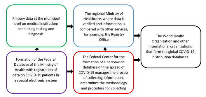
A diagram of the geodata database formation for the spread of a new coronavirus COVID-19 infection in the Russian Federation.
At the regional level, statistical information is received daily from municipal governments, where data is transmitted from health facilities (Figure 1). Since the WHO only provides recommendations for monitoring the spread of coronavirus, data collection and processing systems may vary at the national level, so direct cross-country comparison of raw data without pre-processing is difficult. To investigate the patterns of a new coronavirus infection spread within the borders of different countries, it is desirable to use databases from countries that use similar methods of recording the number of people who became infected, recovered, and deceased as a result of COVID-19 infection when compiling statistics.
For cross-country comparison, a relative indicator of the form F*(t) = N(t)/Nk is used, where N(t) is the number of cases at the time t (the day from the beginning of the pandemic process on 12/31/2019), Nk is the same at the end of the study period tk, which in our case includes time intervals (waves) of the first and the subsequent stages of the pandemic before the appearance of the omicron strain of the COVID-19 coronavirus (SARS-CoV-2) with unique features. That led to a sharp spike in the incidence and its rapid cessation, which requires further special quantitative analysis.
Figure 2 shows graphs of the proportion of daily increase in cases of COVID-19 coronavirus by countries of different continents (P(t) = [F*(t + ∆t) – F*(t)]/∆t, ∆t = 1 day) for the period from t0 = 100 days (04/09/2020) up to tk = 650 days (10/09/2021). Depending on the method of collecting and presenting pandemic information, relatively smooth and non-smooth with sharp daily changes in the value of P(t) differ. The graphs show a shift in the position of infection maxima by territories. During the period under review (2 years), four waves of morbidity were identified with a tendency to increase their amplitude.
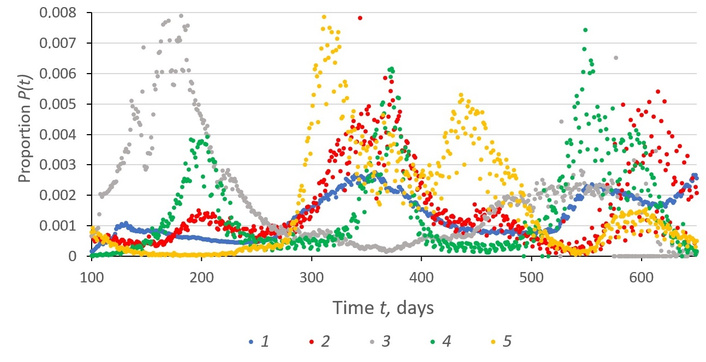
The chronogram of changes in the proportion P(t) of the daily increase in confirmed cases of COVID-19 during the period of 100–650 days of the pandemic by countries. 1—Russia; 2—USA; 3—Saudi Arabia; 4—South Africa; 5—Italy.
There are different types of geoinformational representation of spatial data on maps, reflecting different degrees of penetration into the content of the processes and phenomena under study: analytical, complex, assessment, synthetic, and systemic [26]. When studying and mapping the heterogeneity of population response to coronavirus spread, analytical maps display the spatial variability of initial indicators, which are taken into account in the classical SIR model (number of people who became diseased, deaths, recovered) [15], as well as their relative values (morbidity, mortality, lethality), e.g., the proportions of people who became diseased and died in relation to the total population of the country [1, 27]. Such primary information is usually displayed on the Internet using geographic infographics [22], often with elements of animation and zooming. Comprehensive maps show, with the help of diagrams, the ratio of population proportions belonging to different states of people in the epidemic process. Information for assessment maps is calculated by formulas based on initial indicators, for example, by calculating reliability, hazard, and public health risk values. Synthetic (integral) maps illustrate the circumstances and conditions of the epidemic by region. Synthesis is performed by solving direct and inverse modelling and mapping problems. System maps reflect the parameters of geoinformation models of epidemiological data linkage specific to different territories.
The methods of fiber bundle in differential geometry (Supplementary material 1), as well as reliability theory (Supplementary material 2), are used as a basis for mathematical modelling and statistical data analysis.
The SIR model [15] describes the redistribution of the number of susceptible (S), infected (I), recovered (R), and differentially removed from the epidemic process parts of the whole susceptible population S0, e.g., the number of recovered patients. Unfortunately, the resulting logistic curve of the solution function of the SIR equations does not fit well with statistical plots of the development of a new coronavirus pandemic by country [28], and new equations for modelling need to be sought. A promising direction of modelling in this area is the relations of probability and reliability theory [17, 18].
Processing of geodata by Equation S7 is provided by its reduction by the hierarchy of principal fibrations G{G[f(y)]} → G[f(y)] → f(y) to the linear form f(y) = K(τ). The probability equations F*(z) for the occurrence of extreme values z of different types have the general form Equation S7 for maximum and minimum values τ = t and τ = θln(t/tm) + tm. For Equation S7, the integrated hazard E*(τ) = –lnF*(z) = exp[–α(τ – τm)]and the risk (failure rate) p(τ) = –dE*(τ)/dτ = αexp[–α(τ – τm)], where p(τm) = pm = α is the acceptable risk (AR). The value ln[–E*(τ)] = –α(τ – τm) depends linearly on τ. The dependence K(τ) = –α(τ – τm) is a functional analogue of the universal Equation S2 when f(y) = K(τ), y = τ – τm, i.e., the value τ = τm corresponds to the point of tangency of the line K(τ) of the envelope manifold F(τ). The tangent K(τ, τm) to F(τ) at the new point τ = τm is the layer in which the distribution F*(z) = exp{–exp[K(τ, τm)]} with individual parameters (τm, α) is formed. When τm changes, a path on F(τ) is constructed along which K(τ, τm) changes and the transition from one function of F*(z) to the other takes place.
The constant α is the sensitivity of the change K(τ, τm) when τ changes, which determines the value and direction of the vector α individually in each layer of K(τ, τm) [21] (Figure 3). Content-wise, pm = α = ePm = eVm/S0 is determined by the value of the extremum (peak) of the distribution density function, increases with the maximum of the current incidence increase Vm and decreases with increasing infection potential S0, varying across countries. The values of (τm, α) vary from place to place, preserving the general (true) form of the functional dependence P(τ, τm) with parameters (τm, α).
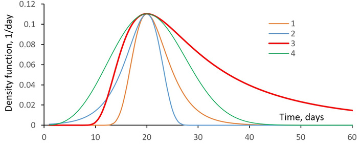
Different types of density function curves for maximum and minimum values. 1–2—Gumbel’s function, 3–4—Fréchet function with the same parameters α = 0.3/day, τ0 = 20 days, θ = 9 days.
The appearance of equations of the form (Equation S7) is associated with the description of the self-regulation mechanism of the infection spread in indicators of integrated hazard:
i.e., the values of differential p(τ) and integrated hazard E*(τ) are proportional to the AR factor pm = α. The steady decrease of E*(τ) with the time course τ is governed by the current infection hazard E*(τ):
When E*(τ) = –lnF*(τ) ≈ 1 – F*(τ) = P*(τ) and F*(τ) = I(τ)/S0, P*(τ) = S(τ)/S0; A = α/S0 = eVm/S02 is the frequency of population contacts. In addition, Equation 1 is a variant of the universal Equation S2 presented in the form of
Statistical graphs of the daily increase in the number of confirmed cases of COVID-19 coronavirus infection grow rapidly at the beginning, reach a plateau, and then slowly decline (Figure 2). Of the curves of the considered functions (Figure 3), the Gumbel and Fréchet distribution functions (Equation S7) of maximum values qualitatively satisfy these features. The last one is convenient because by varying θ in the calculation of the variables of proper time τ = θln(t/tm) + tm, it is possible to increase the size of the plateau of the curve of the epidemic development process. When comparing statistical and theoretical curves [19], the Fréchet function is favoured as more general and adequate according to the similarity criteria, and also because of the fact that in the vicinity of the epidemic peak t = tm the value τ = θln(t/tm) + tm ≈ θ[t/tm – 1] + tm = θ(t – tm)/tm + tm = (θ/tm)(t – tm) + tm depends linearly on time and at θ = tm coincides completely with the time course τ = t, and the Fréchet function with the Gumbel distribution. The relation η = θ/tm indicates the degree to which the situation under consideration corresponds to this ideal case.
For the first wave of the 2020 pandemic in Russia in MS Excel spreadsheets according to the algorithm of description of the statistical graph of daily increase in the number of infected people, the moment of the beginning t0 = 67 day of 2020, when S(t0) ≥ 10 established cases of infection, and the end tk = 240 day of the first (spring) wave of the epidemic [local minimum on the graph S(t)] were distinguished. The value S(tk) = S0 = 975,576 people is considered the potential for infection. The unreliability index is calculated—the probability of health loss of the sensitive population S0: F*(t) = S(t)/S0. We calculate the density of distribution of infection moments—the share of daily increase of sick people P(t) = F*(t + 1) – F*(t) and other reliability indicators (Equation S1): integrated hazard E*(t) = –lnF*(t), risk p(t) = E*(t + 1) – E*(t). By graphing P(t), the mode of the distribution is approximately determined—the moment of epidemic peak tm = 149 days, the maximum value of Pm = P(tm) = 0.0097/day and the AR α = ePm = 0.0264/day. The proper time course is calculated τ = θln(t/tm) + tm at θ = tm. Using Equation S7, approximating curves of the distributions P(t) and P(τ) over time t and τ are calculated by varying the parameters tm, Pm and to θ ensure similarity in terms of correlation coefficient R. The Fréchet function of the marginal distribution at η = θ/tm = 130/149 = 0.87 gives a better approximation (R = 0.95) of the data than the Gumbel function (R = 0.89).
To calculate the proportion of confirmed cases of COVID-19 in Russia Pk(t) (Figure 4) for each epidemic wave k, Equation S6 is applied in real time τ = t with Kk correction for the wave amplitude: Pk(t) = KkP(t). The coefficients of the equation are α = 0.0217 and Pm = 0.008. The location of the seasonal peaks τm = tmk of the proportion of infected people differs by about 179 days, i.e., half a year. For forecasting, it is necessary to know in advance the value of Kk and the location of tmk (modal values) of infection peaks, which is approximately determined by their growth trends: tmk = 170k, Kk = 0.139k. As a result, it is possible to calculate epidemic curves (Figure 4) based on Equation S6 P(t) = Pk(t)/Kk with corrections for the amplitude of Kk and the location of tmk peaks of epidemic waves.
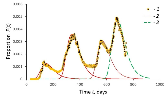
Daily change in the proportion of COVID-19 confirmed cases in Russia. 1—initial data; 2—curves of data approximation according to Equation S6 when τ = t; 3—forecast of changes while maintaining the pandemic situation.
In order to generate the basic parameter maps of the model (Equation S7), a table of coefficients of the Fréchet equation for the distribution of identified cases by country is generated (Table 1). The values α = ePm are obtained to be the same across countries. This means that the pandemic across countries belongs to the same type of phenomenon, and there is a line P(tm) = Pm = 0.0947/day enveloping the territorial P(t) functions from above. The curves of the P(t) functions differ in the timing tm of the peak of the P(t) = P(tm) = Pm wave of the epidemic and its duration θ. The morbidity by country (layers, precedents) on the map forms peculiar time-shifted fields of infection spread. Increasing the value θ of the relative rates of proper time τ leads to a reduction in the duration of the epidemic period Δt0 = t0 – tk in a country, which also individualizes the process, and on the other hand, allows meta-analyses to bring the dependencies P(t) to one typical model with constant coefficients.
Comparison of the parameters of the Fréchet density function for the statistical graphs of the number of COVID-19 cases diagnosed per day in some European countries during the first wave of the pandemic in 2020.
| Country | S0 | t0 | tm | tk | θ | R | η |
|---|---|---|---|---|---|---|---|
| Austria | 16,731 | 61 | 85 | 152 | 530 | 0.95 | 6.24 |
| Belarus | 69,516 | 64 | 130 | 229 | 200 | 0.97 | 1.54 |
| Finland | 7,294 | 65 | 99 | 194 | 159 | 0.80 | 1.61 |
| Germany | 187,226 | 55 | 89 | 164 | 431 | 0.94 | 4.84 |
| Hungary | 4,086 | 71 | 105 | 172 | 275 | 0.77 | 2.62 |
| Italy | 243,230 | 52 | 84 | 195 | 226 | 0.98 | 2.69 |
| Netherlands | 50,834 | 62 | 100 | 187 | 220 | 0.86 | 2.20 |
| Norway | 8,977 | 60 | 84 | 193 | 270 | 0.88 | 3.21 |
| Poland | 35,950 | 68 | 127 | 187 | 61 | 0.79 | 0.48 |
| Romania | 19,398 | 67 | 103 | 153 | 200 | 0.86 | 1.94 |
| Russia | 975,576 | 67 | 149 | 240 | 130 | 0.96 | 0.87 |
| Sweden | 33,188 | 59 | 114 | 144 | 106 | 0.84 | 0.93 |
| Switzerland | 30,871 | 59 | 85 | 153 | 348 | 0.94 | 4.09 |
| United Kingdom | 285,279 | 39 | 101 | 183 | 198 | 0.97 | 1.96 |
Figure 4 shows the first four waves of the COVID-19 epidemic in Russia over two years: observed data and forecasted calculations of the population’s response using Equation S6. The calculations (dotted curve of Figure 4) were performed at the time of 10/25/2021 (666 days of observation) and were confirmed by the current statistics on COVID-19 cases until the beginning of January. However, from 01/14/2022 (day 747), the trend was broken due to the emergence of a new omicron strain of COVID-19, whose epidemic is radically different in terms of both the time of onset and the scale of manifestation, and requires a special study.
A thematic model of the COVID-19 pandemic process developed using reliability theory is used to test scientific hypotheses through meta-analysis. This involves statistical identification and mapping of how populations in different countries respond to the anti-epidemic measures of public authorities in order to manage the risks of infection.
In order to combine the results of studies from different territories, to support and test scientific hypotheses, we propose using meta-analysis methods [20]. They are applied to the assessment of the population response of different countries to the spread of the COVID-19 disease. It allows us to identify the general regularities of the epidemic process [18] and to present them in the form of a mathematical model of its gradual development in order to solve direct and inverse problems of modelling and forecasting the emergence of crisis situations.
Meta-analysis is a set of procedures through scientific methodology, which consists of combining the results of a number of studies using statistical methods to test one or several interrelated scientific hypotheses. Meta-knowledge is pure knowledge abstracted from local circumstances, territorial peculiarities. The high generality of the approach, its interdisciplinary character, and consideration of environmental conditions allow us to consider the methodology of meta-analysis at the meta-theoretical level, which implies the use of mathematical formulas for knowledge representation with fundamental substantive constraints [20]. Meta-analysis is most widely applied in the social, medical, and biological sciences [29–31], where it is used to identify common patterns, to explore and explain observed differences due to heterogeneity of study results, and thus to increase the accuracy of the assessment of intervention effects through statistical processing of the available information. This allows a more precise definition of the categories of objects and types of environments for which the results obtained are applicable [20].
The methodology of meta-analysis is based on a meta-theoretical framework—the hypothesis of systemic stratification of Earth reality on the diversity of geohistorical environment. Locally, processes and phenomena are described by homogeneous Equations S1 and S2 of data integration, so each situation is reduced to the properties of the type layer and universal equations f(y) of the variables’ relationship [20]. This allows understanding and investigating different objects as the same object, and matching them by comparing them with a chosen etalon.
Reliability functions are analytically related to P*(t) and to each other according to Equation S3, therefore, specifying one of them, we obtain all the others. For example, F*(t) = exp[–E*(t)] is the unreliability, which exponentially increases with decreasing hazard. In particular, it reflects the relative increase in the number of infected with decreasing risk of getting infected at the last stages of the pandemic. The meta-dependence p(τ) = αE*(τ) + ε is reliably manifested in the Russian Federation population response and satisfies Equation 1 p(τ) = 0.0217E*(τ) – 0.0169 with a correlation coefficient R = 0.919.
For the Fréchet function, the following relation is correct
Equation 4 in E*(τ) coordinates does not depend on the environmental parameters (τm, α), so it can be used in the process of meta-analysis to highlight general patterns.
According to Equation 4, the normalized value ρ(τ) = P(τ)/Pm should ideally be determined only by the integrated hazard E*(τ). For the individual epidemic wave curves, this value is transformed E*(τ) → e*(τ) for each country so that the plots pass through the origin (0, 0) when the normalised value e*(τ) = 0 and the maximum point (1, 1) when P(τ)/Pm = 1 and e*(τ) = 1. The transformation e*(τ) = [1.61E*(τ) – 0.78]λ, λ = 1.45 common for all countries shows that the dependence (Equation 4) linear at λ = 1 is generally non-linear λ = 1.45, i.e., there is an interaction of hazard indicators E*(τ), which is usually associated with a positive effect of self-organization.
The graphical dependence ρ(τ) = P(τ)/Pm on e*(Figure 5a–b) of the observed values for individual countries corresponds to the calculated curve ρ[e*] of the Equation 4. The similarity of Pn(e*) plots for the population of different countries (Figure 5b) is revealed, which allows us to consider various dependencies (Figure 5a–b) as a single meta-law, which satisfies Equation 4 for normalized values of E*(τ) → e*(τ) and accounts for 94% of the points on the graph. For Russia, the similarity between the empirical and theoretical indicators of the dependence ρ[e*] is very high (Figure 5a, R = 0.97).
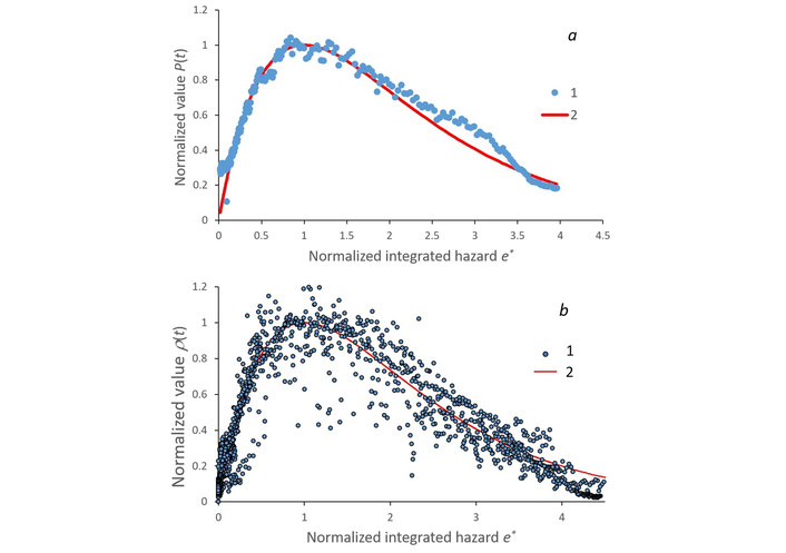
The dot plots of the dependence of the normalized proportion ρ = P(τ)/Pm of confirmed cases of the second wave of COVID-19 on the value of e*(τ) of standardized integrated hazard E*(τ): (a) in Russia, (b) as well as with overlapping graphs of different countries (Russia, USA, South Africa, Mexico, India, Kazakhstan, Canada): 1—initial data; 2—the curve of data approximation according to Equation S7. Calculated based on data from [22].
In the course of meta-analysis, the information is compressed. Constant coefficients and general regularities of the relationship between the characteristics of systems are identified in a ‘pure’ form in the central informative part of the data series of one wave. The minimum scatter (homogeneity) of data around the graphs of theoretical formulas determines the reliability of connections and allows their use in different conditions for processing data series and solving forecasting problems. The graphs in Figure 5 confirm the applicability of Equation 4, and thus of Equations S5 and S6 in statistical studies, but do not necessarily justify them definitively, because the recommended form of the Equation E*(τ) may be different H: F*(τ) → E*(τ) = H[ln(F*(τ))] → K(τ) = H[ln(E*(τ))], which requires clarification.
The spread of COVID-19 disease is considered an emergency pandemic situation, dangerous for the population and economy of states. Ensuring the safety of global and regional life systems requires prompt analysis of incoming information about the epidemic process of infection and the creation of adequate models and methods of risk management [17]. The complexity of the proposed hierarchical models is expressed in the multiplicity of the embedding (superposition) of exponential functions G{G[f(y)]}. In the epidemic model, this is managed by reducing the value of the AR α of infection through organizational pressure on the value of this risk α = f(y). The effectiveness of the pressure is assessed by the values of sustainable controllability indicators, individualized for each area.
To describe the reliability function P*(t) of the first wave, Equation 5 in the z = α(t – tm) variant of the Gompertz Equation [17] was used:
where P(tm) = Pm is the largest value of the function P(t). AR α defines the safety boundaries of existence of the considered system at t = tm, when the distribution curve P(t) reaches its maximum P(tm). According to Equation S1, the failure rate is equal to p(t) = αE(t), from which the coefficient α = p(t)/E(t) is calculated, even if it has a variable value α(t).
At the first hierarchical level, the exponential hazard function E(t) = αexp[α(t – tm)] is manifested, and at the second level, the twice-exponential reliability function P*(t) (Equation 5). By analogy, at the zero level of complexity, we should expect an exponential dependence of AR α(t) (the riskiness of the situation) on time:
where αm is the limiting value of AR (t → ∞); β is a constant control coefficient of AR reduction. In Equation 6, the value of g = α0β is the strength of the control pressure on the development of the epidemic process (controllability); χ = α0 + gtm + αm is the AR value at the very beginning (t = 0) of the global pandemic manifestation in a given country. The coefficient χ is an indicator of the unpreparedness of the state and society for the epidemic, which is positively determined by the value of gtm, starting α0 and final αm level of AR. Obviously, preparedness increases with increasing manageability β, later moment of epidemic peak tm and a higher value of AR allowed in the country at the beginning α0 and at the end αm of the process.
The statistical materials available at the end of May 2020 were processed by numerical methods using the given equations. The inverse problem of modelling—determination of informative model coefficients using time series data—was solved. The epidemic curves were compared across countries to find out the functional complexity of the process under study in each area.
The exponential increase in AR (Equation 6) corresponds to a linear dependence of lnα(t) on time t with an individual offset tm at the beginning of the epidemic process (R > 0.98) (Figure 6). Calculations for Italy give the ratio ln[α(t) – αm] = –0.0355(t – 18.0) (R = –0.97), αm = 0. Then we get α(t) = exp[–0.0355(t – 18.0)] (R = 0.97), where the controllability index β = 0.0393. The initial AR was highest in China (α0 = 0.267) and lowest in Russia (0.194). In Western countries α had a close value of 0.243. The value of 1/α0 indicates the degree of preparedness of a country’s health care system for a pandemic.
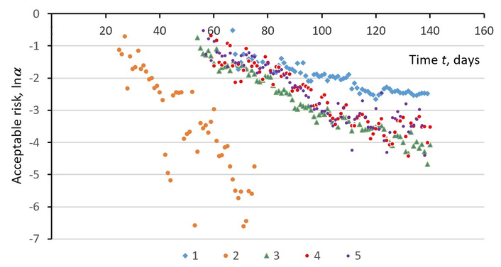
Changes over time in the AR lnα(t) of the COVID-19 coronavirus epidemic in some countries. 1—Russia; 2—China; 3—Italy; 4—Germany; 5—Spain.
On the basis of the models, the peculiarities of the population response of different countries to the actions of state authorities in managing the risk of infection through their influence β on the value of AR α. Sustainable indicators (parameters) of controllability β, individual for each territory, become characteristics of the impact efficiency. The authorities of China demonstrated high manageability of the population in the conditions of the beginning of the epidemic, the average level is typical for Western countries, and the Russian population showed low manageability with high state readiness for the pandemic. The territorially close countries—Italy, France, and Spain—showed similar trends of pandemic development with slightly different coefficients of Equation 6 (Figure 6).
The comparative analysis of reliability functions [19] makes it possible to identify the Fréchet distribution Equation S7 as the best approximation of F*(t) curves. This equation uses multilevel independent variables t, τ, z, and their functions F*(t), F*(τ), F*(z), with the same values F*(t) = F*(τ). Equation S7 reflects the probability F*(z) of occurrence of extreme (maximum) values of z[τ(t)], associated with moments t of detection of failures from normal (healthy) functioning (facts of disease)—the proportion of those who became infected and re-infected out of the number of those susceptible to infection during time t from the beginning of the epidemic. The rate of change of F*(z) in time P(t) = dF*(z)/dt = (dF*(z)/dz)(dz/dτ)(dτ/dt) corresponds to the daily increment of disease cases—the density function of the failure distribution (disease incidence) (Figure 2), i.e., it shows the excess incidence of new coronavirus infection. The value of the AR coefficient α is found by the position τ = τm = θln(tm/tm) + tm = tm, z = 1 of the maximum P(tm) = Pm of the function P(t): α = ePm, τ(tm) = tm. The value calculated from the data is α = ePm = 0.0264/day [19].
The integrated hazard (threat, possibility of getting infected by time t) is calculated by the Equation E*(τ) = –lnF*(z) = exp[–α(τ – τm)] and the risk of disease p(τ) = –dE*(τ)/dτ = αexp[–α(τ – τm)]. In model Equation S7, the indicator K(τ, τm) = ln[E*(τ)] = –α(τ – τm) depends linearly on τ and is the functional analogue of the universal Equation S2 with f(y) = K(τ, τm), a = –α, y = τ – τm. At the same time, the modelling problem can be set in the general form f(y), taking into account the influence of various environmental factors y = x – x0 on the hazard indicator K(x, x0) = f(y). An example is the Cox model [32] of risk assessment p(x) of an event occurrence taking into account the influence of independent variables (predictors) x = {xi}.
The calculated values of K(τ, τm) are well approximated by a linear dependence on time t (Figure 7):
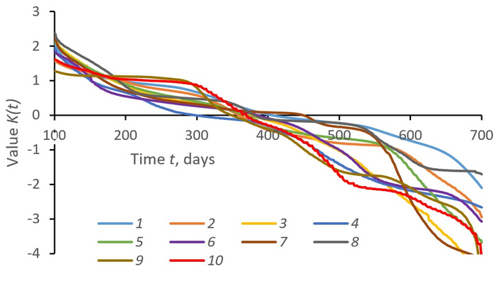
The variation in time t of hazard indicator K(t, tm) = lnE*(t) of population infection with coronavirus in different countries. 1—Russia; 2—USA; 3—Brazil; 4—Peru; 5—Mexico; 6—Chile; 7—Bangladesh; 8—South Africa; 9—Italy; 10—Sweden.
Here, the ratio of the coefficients γ = αθ/tm individually parameterises the epidemic process in different countries. The linear Equation 7 reflects the general trend of increasing K > 0 and decreasing K < 0 morbidity without taking into account periodic fluctuations (epidemic waves). The values τm, γ vary from country to country are unique to each country.
The linear regression coefficients a and b are statistically estimated:
According to the difference of a and b by countries, it is possible to estimate the peculiarities of epidemic processes and to display them differently on cartograms, in particular, according to the value of a = –γ—about AR a = –β = –aθ/tm, and according to the values of b = βtm = αθ—about the optimality of the management of the infection process: the smaller b—the more effective the preventive and anti-epidemic measures, the results of which are revealed during the period T = 100 ÷ 650 days.
Territorially, the values θ = b/α and tm = –αθ/α vary, indicating the optimality and environmental conditions of the epidemic process realisation. Coefficients a and b of Equation 8 vary by country, for example, for Russia K = –0.00488t + 2.06 = –0.00488(t – 422.9) (correlation coefficient R = –0.98), for the USA K = –0.00625t + 2.26 = –0.00625(t – 362.1) (R = –0.98), for Brazil K = –0.00929t + 3.09 = –0.00929(t – 332.6) (R = –0.96). In Russia, γ = 0.00488/days, tm = b/γ = 422.9 days, the proper time value θ = γtm/α = b/α = 78.1 days. The value of tm indicates the moment of culmination of the epidemic process, when K = 0 and the hazard has a critical value E*(tm) = 1. Later tm dates characterize the best pandemic situation in terms of disease spread: Russia—423 days, South Africa—400 days, Germany—247 days, etc.
The value θ = b/α is proportional to the free term b of the regression Equation 8, so its increase indicates a worse quality of management of the epidemic process, which lasts longer. Of the countries studied, the best by this criterion are Saudi Arabia and Russia (θ < 80 days), while the worst (θ > 110 days) are Brazil and Sweden, which have been noted in the press as countries with low intensity of government pandemic management. The time indicators tm and θ are not correlated (R = 0.02), so they can be used as independent indicators for mapping (Figure 8).
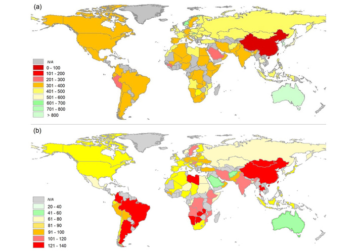
Global change of the mathematical model parameters of the population response of different countries to COVID-19 infection: (a) the moment tm (number of days) of the epidemic process peak; (b) the index θ (number of days) in the proper time.
In geoinformation mapping, the indicator method is implemented [33] when the unknown system status is identified by a set of indicators using a formulaic integrating estimation, which gives a graphical or cartographic representation informing the user about the required state. Graphs and mappings are used to compare indicators (signals)—individual parameters of a mathematical model of the system’s behavior—with each other and with limit values. In this case, the indicator method is implemented by estimating the parameters of the dependence K(t, tm) = –(αθ/tm)(t – tm) (Equation 7).
The presented cartograms are filled with the results of calculations for countries for which statistical information is available. On the basis of this information, it is possible to estimate the values of tm and θ, and to calculate the coefficients of Equation 8: α = –γ = –αθ/tm, b = –αtm = αθ, and then calculate K = K(τ(t), τm) = at + b, E*(τ) = exp[K(τ, τm)], F*(z) = exp[–E*(τ)] in order. Thus, the set of cartographic geo-images-cartograms (Figure 8) reflects integral (synthetic) properties of the population response of different countries to COVID-19 infection, which is described by the equation of the corresponding mathematical model Equation S7, according to which derived indicators of the reliability of public health preservation can be calculated and then analytically mapped.
Of the processed spatial data on coronavirus epidemics in 86 countries, in 95% of cases, they satisfy the linear Equation 8 with a coefficient of determination R2 > 0.90. The tm values reflecting the moment of maximum coronavirus morbidity trend are concentrated in the interval of 300–500 days. They are shown on the cartogram in steps of 100 days, dividing this interval into two parts with different lags of pandemic deployment by country. The values of θ of the proper time course indicators are mainly located in the interval 60–100 days and are shown on the cartogram with a color scale interval of 20 days. The best indicators of a country’s healthcare system for managing the pandemic process are shown in green on the cartograms, while the worst are shown in red.
The extreme events associated with the spread of COVID-19 infection among populations in different countries provide information from a variety of sources for comparative analyses and quantification of the quality of decision-making in different national pandemic control situations. Societies and people in different regions and countries react differently to the spread of the epidemic, because it is difficult to accurately reproduce its development in mathematical models and offer optimal solutions to real epidemiological problems [34].
It has been found that the traditional SIR epidemic model, with constant parameters, is not sufficiently accurate to describe the transmission of infectious diseases across different countries. This has been confirmed by other studies [28, 34–38], which have shown the need for further additions and modifications to the model. It still needs to be improved and further developed based on the latest information about the COVID-19 infection [39, 40]. It is also suggested to use probabilistic models to approximate morbidity curves, including reliability functions [17, 18, 41, 42]. Comparative statistical analysis reveals that the Fréchet function is the best option, with its rapid growth and gradual attenuation of the infection wave.
Using mathematical models of reliability theory, the general trend of the epidemic curves is identified. The coefficients of the models and the dynamics of the number of established cases of disease as a function of failures (facts of infection), probability density of failures (increase in the proportion of infected), integrated hazard and risk of infection, AR, primary epidemic preparedness, and manageability of the current epidemic situation are promptly calculated. The basis for mathematical and statistical analysis is the exponential hazard equation, which, on a logarithmic scale, is represented by a linear dependence on time. Its variation by changing the controlled value of AR reveals national differences in epidemic load regulation among the population. All reliability indicators have clear meanings and are interconnected. For forecasting purposes, it is essential to know the moments of the beginning and peak of the epidemic, the potential for infection in the risk group, and AR levels.
The statistical function of failure density, i.e., the proportion of cases identified per day, shows the relative deviation from the public health norm (excess morbidity). By stratifying the linkage function of the observed variables, a self-perpetuating epidemic process is modelled, stretched in its proper time, and implicitly managed through protective measures, which is reflected in the model parameters for each country and in the mapping of unique management performance indicators for different countries.
The methodology for space stratifying (fiber bundling) on the diversity (manifold) of linkages of population response indicators of the COVID-19 pandemic in different environments was used in the paper. The comparison of systemic links across fiber layers (countries) in the meta-analysis process is done in such a way that different systems are represented as one, in order to identify common patterns, beyond local conditions and territorial specificities. The Fréchet function is used to represent each country by an epidemiological curve with individual coefficients. Subsequent country comparisons were made by comparing the position of epidemic wave peaks and their amplitude. It has been revealed that the general population in different countries responds similarly to the situation according to a single law of self-regulation of the risk of infection, despite differences in socio-economic, natural-climatic, political, and other factors of coronavirus spread. Thus, the proposed scheme of meta-analysis of spatial and temporal epidemiological data on COVID-19 allowed us to identify invariant dependencies unrelated to territorial specificities of virus spread.
On the basis of the models, we have assessed the specifics of the population response in different countries to the actions of public authorities to manage the risk of infection through their impact on the value of AR. Sustainable indicators (parameters) of manageability, individual for each country, become the characteristics of the impact efficiency. The authorities of China demonstrated a high level of manageability of the population in the conditions of the beginning of the epidemic, the average level is characteristic of Western countries, and the Russian population showed a low level of manageability with a high level of state preparedness for the pandemic. The territorially close countries—Italy, France, and Spain—showed similar trends in the development of the pandemic, with slightly different equation coefficients.
The suggested model describes the trend of change in the population response of different countries to the spread of the coronavirus, taking into account the geographical heterogeneity of the parameters of the model equations, realizing that each contour of the cartogram hides specific information for the construction of estimation and forecasting cartograms based on this model. Such heterogeneity depends on the peculiarities of state epidemic regulation and the stages of global pandemic deployment. The complexity of system mapping procedures increases with the improvement of GIS-modelling methods aimed at identifying universal and unique characteristics of the phenomena under study, in this case, to further take into account in one formula of integrated hazard and reliability the observed periodic component of epidemic processes throughout the pandemic.
Although this article focuses on identifying hidden laws and patterns in terms of reliability theory, it also has practical value in assessing the country-specific response to the pandemic. The article examines how the population and government have reacted to the development of the pandemic in different countries. The results of the study can be used to compare countries in terms of how their societies respond to the spread of disease, to quantitatively analyze mass behavior in critical situations, and to understand the uniqueness of each nation. It is possible to offer recommendations for improving preparations for a pandemic, addressing its consequences, and managing the population’s behavior during an epidemic in isolation and vaccination mode. Comparison with reference curves allows us to assess the accuracy of the initial state and regional statistics. Finally, based on the outcomes of the pandemic, there is an opportunity to determine the extent of historical responsibility for the consequences of the pandemic.
Of particular importance for theoretical research is the finding about the central role of the dimensionless quantity of the integrated hazard in the quantitative analysis of time series. It can be used for extrapolating and interpolating data, as well as solving forecasting problems. The existence of a logarithmic proper time scale has been confirmed, on which the effect of self-regulation in processes can be clearly seen. There is a connection between this and the exponential Cox model [32]. The model is expressed in transformed variables and is used to study how the risk of an event depends on the duration of a person’s time in a risk group.
However, there are some areas that need further improvement in the model. Specifically, it does not account for the periodic nature of the pandemic, and the meta-analysis data suggest the need to refine the basic reliability equation. It is important to consider the territorial interaction and spread of the disease among populations in different countries as a unified global process. It is necessary to reflect in the appropriate formulas the reasons for the sudden onset and end of the pandemic in our analysis. It is important to consider the influence of various external factors, both natural and social [43–45], which can affect the values of the coefficients in the mathematical model that describes the population’s response to COVID-19 infection in different countries (see Figure 8).
It is possible to apply the methods of reliability theory, in the accepted interpretation, to solve other problems that are being tested and developed using this approach [46, 47]. This technique, in particular, is used to create a cartographic model of the heterogeneity of a geo-field based on cartographic data. The altitude distribution of geosystems, in terms of the occurrence Pi(x), is the density (calculated per 100 meters) of the probability of finding an i-type geosystem in a given vertical range x [48, 49]. The research we conducted has provided interesting and encouraging results. This allows us to draw some general conclusions about the methodology. We can study changes in reliability functions in both temporal and spatial dimensions, as well as in indicators of the state of a system, such as levels of public health or environmental quality.
In this regard, the generalized McKendrick-Von Foerster first-order linear partial differential equation is interesting in its application to biomedical research [50, 51]. The equation describes dynamic flows that are characteristic of modeling phenomena in a continuous medium [52, 53], and it has generalized forms for describing changes in functions of multiple variables. We believe that the general Equation 2 of pandemic self-development in this case can be expressed as a partial differential equation for changes in the integrated hazard simultaneously in time, age, and other aspects of the situation, leading to accurate mathematical transformations, such as Lagrange’s substantial derivative in the study of open complex systems [54].
The periodic and discrete nature of the distribution and magnitude of danger is reflected in second-order quantum partial differential equations [55–57]. These equations will further help us to understand the hidden nature and specific characteristics of epidemic processes across countries and continents. Having worked on numerous examples of the use of reliability theory methods in modeling and statistical processing of spatial and temporal data series, we have identified important patterns. Based on these findings, we can confidently and meaningfully apply the results in biomedical research, modeling, and healthcare practice, including in the fight against pandemics.
AR: acceptable risk
GIS: geographic information system
SARS-CoV-2: severe acute respiratory syndrome coronavirus 2
SIR: susceptible-infected-recovered
WHO: World Health Organization
The supplementary materials for this article are available at: https://www.explorationpub.com/uploads/Article/file/101168_sup_1.pdf.
AKC: Conceptualization, Methodology, Formal analysis, Software, Writing—original draft. NEK: Investigation, Formal analysis, Writing—original draft, Writing—review & editing. Both authors read and approved the submitted version.
The authors declare that they have no conflicts of interest.
This manuscript presents a re-analysis of publicly available datasets that are fully anonymized and do not contain any personally identifiable information. Therefore, ethical approval is not required under the guidelines of the V.B. Sochava Institute of Geography.
This manuscript presents a re-analysis of publicly available datasets that are fully anonymized and do not contain any personally identifiable information. Therefore, consent to participate is not required under the guidelines of the V.B. Sochava Institute of Geography.
Not applicable.
The datasets of the COVID-19 spread analyzed for this study were obtained from open sources on the websites of Johns Hopkins University (https://coronavirus.jhu.edu/about/how-to-use-our-data), the World Health Organization (https://data.who.int/dashboards/covid19/cases), and Worldmeters (https://www.worldometers.info/coronavirus/).
The work was supported by the Russian state assignment AAAA-A21-121012190056-4. The funders had no role in study design, data collection and analysis, decision to publish, or preparation of the manuscript.
© The Author(s) 2025.
Open Exploration maintains a neutral stance on jurisdictional claims in published institutional affiliations and maps. All opinions expressed in this article are the personal views of the author(s) and do not represent the stance of the editorial team or the publisher.
Copyright: © The Author(s) 2025. This is an Open Access article licensed under a Creative Commons Attribution 4.0 International License (https://creativecommons.org/licenses/by/4.0/), which permits unrestricted use, sharing, adaptation, distribution and reproduction in any medium or format, for any purpose, even commercially, as long as you give appropriate credit to the original author(s) and the source, provide a link to the Creative Commons license, and indicate if changes were made.

View: 1686
Download: 107
Times Cited: 0
Ashrafe Alam, Victor R. Prybutok
Ard Hendriks ... Sil Aarts
Kun Li ... Visara Urovi
Yuyang Yan ... Visara Urovi
